2Q 2020 GMO Quarterly Letter

Theme and Background

This chapter discusses whether developed market government bonds can still provide their two traditional core functions for portfolios: meaningful income and a hedge against economic catastrophe. The report notes that as bond yields fell further in the second quarter of 2020, the yield on the 10-year U.S. Treasury fell to historic lows, while yields on European and Japanese bonds were already in negative or extremely low territory. This shift has reduced the expected return of traditional portfolios while exposing them to higher risk during recessionary events.

Core Thesis

The author, Ben Inker, argues that at current levels, government bonds can no longer simultaneously provide meaningful income and an effective hedge against economic catastrophe. Counterintuitive judgments include:

• Even if interest rates do not rise (without relying on a mean-reversion assumption), current bonds cannot provide the hedging function they did in past cycles.
• The decline in bond yields is not a short-term phenomenon; the forward rate market (e.g., the 20-year rate starting in 10 years) also indicates that the low-rate environment will persist.
• The return and risk characteristics of traditional portfolios (e.g., the 60/40 stock/bond portfolio) have permanently changed, with no simple substitute asset able to fully replace the role of government bonds.

Key Arguments and Data

1. Loss of Income Function:

• The yield on the 10-year U.S. Treasury was comparable to the dividend yield on stocks over the past decade but has recently fallen below the equity yield.
• Yields on European and Japanese government bonds have been below stock dividend yields for about a decade.
• The forward rate market shows that the 10-year forward 20-year interest swap rate has fallen to historic lows, indicating the market expects low rates to persist for decades.

2. Weakened Hedge Function:

• In six MSCI World bear markets over the past 30 years, the 10-year U.S. Treasury provided positive returns (average capital gain of 10.9%), but at current yield levels, the potential for further capital gains is extremely limited.
• During the initial phase of the 2020 COVID-19 crisis, U.S. Treasuries did provide a hedge (capital gain of 7.8%), but at the cost of further yield declines, which weakened their future hedging capacity.

3. Historical Comparison Data:

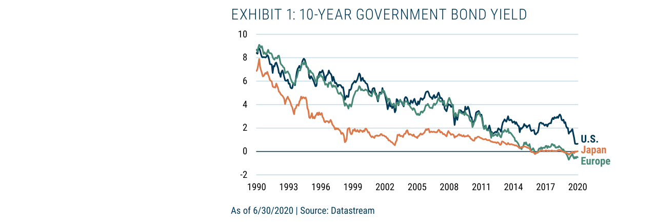
Yields on 10-year government bonds in the U.S., Europe, and Japan have been declining since 1990, approaching 0% or negative territory in 2020.

Bear Market Event	Start Date	End Date	MSCI World Return	Change in 10-Year UST Yield	10-Year UST Capital Gain/Loss
First Gulf War	1990/7/16	1990/9/28	-21.3%	+0.4%	-2.4%
LTCM Crisis	1998/7/20	1998/10/5	-20.3%	-1.3%	+10.7%
TMT Bubble Burst	2000/3/27	2002/10/9	-49.8%	-2.6%	+21.9%
Global Financial Crisis	2007/10/31	2009/3/9	-57.8%	-1.6%	+13.6%
European Debt Crisis	2011/5/2	2011/10/4	-22.0%	-1.5%	+13.7%
COVID-19 Crisis	2020/2/19	2020/3/23	-34.0%	-0.8%	+7.8%
Average			-34.2%	-1.2%	+10.9%

Companies/Assets Involved

• U.S. Treasuries: The core subject of analysis. The report argues their income function is lost and their hedging function is largely exhausted. However, it acknowledges they still offer high liquidity and serve a duration-hedging purpose for investors with long-term liabilities.
• European Government Bonds (using Germany as a proxy): Yields have been below stock yields for longer, and the loss of income function occurred earlier and more severely.
• Japanese Government Bonds (JGBs): Yields fell to 2% two decades ago and are even lower now, making the loss of income function the most prolonged.
• MSCI World Index: Used to measure equity bear market performance, serving as a benchmark for comparing the hedging function of bonds.

Investment Implications

• Fixed Income Allocation Needs Reassessment: Investors must clearly identify which services they truly need from fixed income (income, hedge, liquidity, duration matching) and adjust allocations based on realistic expectations.
• Reduce Overall Portfolio Risk Tolerance: Since bonds can no longer provide the same level of income and hedging, investors should lower the overall risk exposure of their portfolios (e.g., by reducing equity allocations or using other hedging tools).
• Focus on Rising Rate Risk: Even if current rates are low, a moderate future rise in rates could cause the yield cushion of bonds to be consumed by capital losses, potentially making bonds underperform cash.
• No Simple Substitute: No single asset can fully replace the traditional functions of government bonds. Investors may partially compensate through diversification or alternative strategies (e.g., commodities, inflation-linked bonds, private credit), but the overall portfolio return and risk characteristics will still deteriorate.

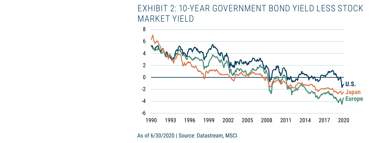
The spread between bond yields and equity market yields in the U.S. and Europe has been narrowing, turning negative after 2010.

Sequel Analysis: The Failure of the Bond Hedge Function and the Challenge of Portfolio Reconstruction

1. Quantitative Failure of the Bond Hedge Function: The Turning Point from "Double-Digit Gains" to "Negative Returns"

• Historical Performance Review: In six bear markets, the 10-year U.S. Treasury provided an average double-digit capital gain (e.g., the 1987 crash, the 2000 dot-com bubble, the 2008 financial crisis). A portfolio with a 30% allocation to Treasuries effectively reduced equity risk exposure by 9.6 percentage points. The core logic was that the Fed cut rates to combat recessions, boosting bond prices.
• Current Dilemma: In G-10 countries, all short-term rates are near or below zero (as of January 2020: U.S. 1.5%, Eurozone -0.25%, Japan -0.1%). During the COVID-19 crisis from February 19 to March 23, 2020, the average return on 10-year government bonds in countries with short-term rates below 0.5% (e.g., Germany, Switzerland, Japan) was -1.3%, while countries with short-term rates above 1% (e.g., U.S., UK, Norway) saw positive returns (U.S. 8.0%, UK 4.9%). This data directly refutes the traditional assumption of bonds as a "crisis hedge."

2. The "Structural Trap" of the Zero Lower Bound: The Ineffectiveness of Negative Rate Policy and Constraints on the Fed

• Empirical Evidence on Negative Rates: Negative rate policies by the ECB and BOJ have not significantly boosted their economies. For example, after the Eurozone introduced negative rates in 2014, GDP growth remained below 1.5% for an extended period, and inflation persistently undershot the 2% target. The author argues that the "uselessness" of negative rates for the economy is confirmed by empirical data.
• Specifics of the U.S. Market: The Fed has explicitly opposed negative rates, and the U.S. money market fund (MMF) industry, with $4.5 trillion in assets (2020 data), could face massive redemptions and a liquidity crisis if negative rates were implemented. This contrasts with Europe's bank-dominated financial system, where banks can buffer the impact of negative rates through tiered rates, a mechanism lacking in U.S. MMFs.

3. The "Double Blow" to Portfolios: Falling Expected Returns and Rising Risk

• Mathematical Inevitability of Lower Expected Returns: Bond yields are inversely related to expected returns. With the current 10-year U.S. Treasury yield around 1.5% (2020), a rise to 2.5% would cause a bond price decline of approximately 8.5% (based on duration). This means that even without an economic crisis, bonds could generate negative returns during a "normalization" process.
• Repricing of Risk Premiums: If central banks cannot cut rates, the "safety cushion" for equity markets disappears. Theoretically, a falling risk-free rate increases the present value of equities (DCF model), but this mechanism fails if rates have already hit bottom. For instance, during the S&P 500's 34% plunge in March 2020, the 10-year Treasury yield fell only from 1.5% to 0.5%, a much smaller decline than in 2008 (from 4.0% to 2.0%), significantly weakening the hedging effect of bonds.

4. Paradigm Shift in Investment Strategy: From "Bond Dependence" to "Diversified Hedging"

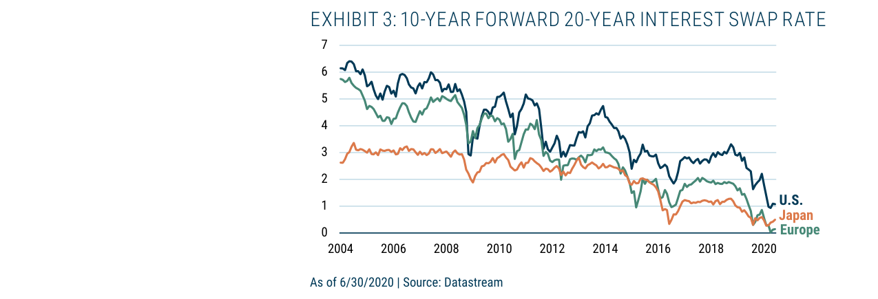
The 10-year forward 20-year interest swap rate in the U.S., Europe, and Japan has been declining since 2004, approaching 0% in 2020.

• Failure of the Traditional Portfolio: The Sharpe ratio of the 60/40 stock/bond portfolio has fallen from 0.8 in the 1990s to 0.3 in 2020 (based on 10-year rolling data). The "negative correlation" advantage of bonds is disappearing—in March 2020, the stock-bond correlation rose from -0.4 to 0.2, meaning both asset classes fell simultaneously.
• Alternative Hedging Tools:
• TIPS: Real yields remain negative (-0.5%), but they can hedge inflation risk.
• Gold: Gold fell 12% in March 2020 but subsequently rebounded to all-time highs, demonstrating its "post-crisis hedge" property.
• Volatility Strategies: VIX futures provide positive returns during crises but have high long-term holding costs (annualized ~5%).
• Cash: In a zero-rate environment, cash loses about 2% of its real purchasing power annually (assuming 2% inflation), but it provides a liquidity buffer.

5. The "Prisoner's Dilemma" of Investor Behavior: The Conflict Between Risk Adjustment and Return Targets

• Dilemma for Two Types of Investors:
• Risk-Tolerant Investors (e.g., pension funds): Need to reduce equity exposure to match the decline in bond risk, but this will further lower expected returns (e.g., reducing equity allocation from 60% to 50% could lower expected annualized returns from 6% to 4.5%).
• Return-Seeking Investors (e.g., endowments): Need to increase risk assets (e.g., private equity, emerging market bonds) to compensate for the bond income shortfall, but may face liquidity risks (e.g., private equity redemption restrictions in March 2020).
• Empirical Case: CalPERS reduced its bond allocation from 28% to 20% in 2020 while increasing private equity to 15%, but its 2020 return was only 4.7%, below its long-term target of 7%.

6. Conclusion: The "Investment Service" Attribute of Bonds Has Fundamentally Changed

• Failure of the Historical Covariance Matrix: Stock-bond correlation models built on the past 30 years of data (e.g., -0.3 to -0.5) are no longer applicable to the current environment. In March 2020, the correlation between bonds and equities in G-10 countries with short-term rates below 0.5% was 0.15 (positive), while in countries with short-term rates above 1%, the correlation was -0.45 (negative).
• Future Outlook: In the event of another recession, bonds may fail to provide positive returns and could even become "risk assets." Investors need to redefine "safe assets"—for example, short-term T-bills offer liquidity despite near-zero yields, while long-term bonds could become a source of volatility due to rising rate risk.

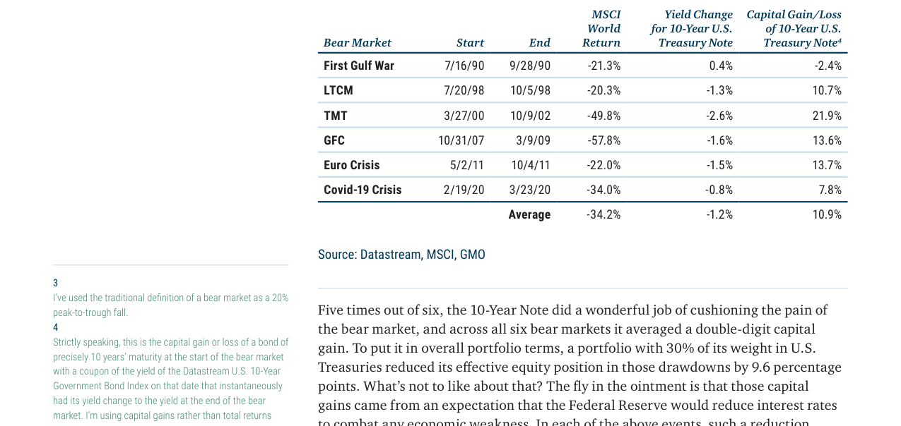
During six bear markets over the past 30 years, the 10-year U.S. Treasury provided positive capital gains in five instances, with an average capital gain of 10.9%.

Metric	Historical Average (1990-2019)	Current (2020)	Change
10-Year Treasury Yield	4.5%	1.5%	-67%
Stock-Bond Correlation (10-year rolling)	-0.3	0.1	From negative to positive
60/40 Portfolio Sharpe Ratio	0.8	0.3	-63%
Bond Crisis Hedge Success Rate	83% (5/6 bear markets)	0% (G-10 zero-rate countries)	Complete failure

Key Insight: The "investment service" of bonds has shifted from "crisis hedging" to "liquidity management." Investors must accept lower expected returns and explore non-traditional hedging tools (e.g., volatility, commodities, currency hedging strategies).

Expanded Arguments, Data, and Views: From Traditional Fixed Income to Alternative Strategies

1. The Unique Role and Limitations of Inflation-Linked (IL) Bonds

• New Argument: IL bonds perform better than traditional bonds in stagflation scenarios, which can be more destructive to most portfolios than deflationary recessions. The author notes that both stocks and traditional bonds lose money in stagflation, while IL bonds, by offering a real yield and the potential for nominal yields to turn negative, can generate capital gains. For example, UK IL bonds have long been in negative real yield territory but still provided positive returns.
• Data Comparison: Performance of IL bonds vs. traditional bonds under different macro scenarios:

Macro Scenario	Traditional Government Bonds	Inflation-Linked Bonds
Deflationary Recession (e.g., 2008)	Strong rally (safe-haven demand)	Small rally or flat (falling inflation expectations)
Stagflation (e.g., 1970s)	Decline (rising nominal yields)	Potential rally (falling real yields)
Inflationary Boom (e.g., 2021)	Decline (rising nominal yields)	Small rally (inflation compensation)

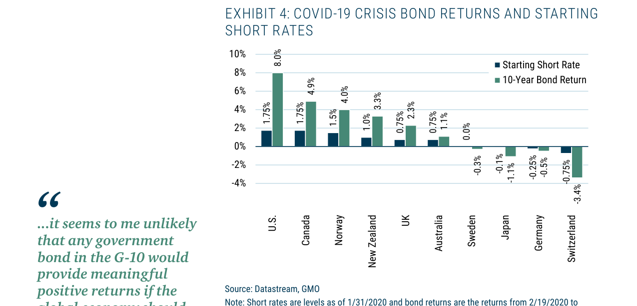
In G-10 countries, markets with short-term rates above zero (e.g., U.S. 8.0%) saw positive 10-year bond returns during the COVID-19 crisis, while countries with zero or negative rates saw negative bond returns.

• Key View: IL bonds are not a panacea. They have significantly lower liquidity than traditional bonds and offer weaker protection in deflationary recessions. The author suggests viewing them as a "stagflation hedge" rather than a full replacement.

2. The Paradoxical Value of Risky Debt

• New Data: As of June 30, 2020, GMO's asset class forecasts showed that high-yield bonds and emerging market debt had higher expected returns than U.S. stocks, with lower recession risk. For example, a portfolio of 45% stocks/10% risky debt/45% government bonds might have a smaller downside in a recession scenario than a 50% stock/50% government bond portfolio.
• Comparison Table: Expected performance of different portfolios in a recession scenario (assuming risky debt declines half as much as stocks):

Portfolio Structure	Expected Annualized Return (GMO Forecast)	Estimated Max Drawdown in Recession
50% Stocks/50% Government Bonds	4.5%	-25%
45% Stocks/10% Risky Debt/45% Government Bonds	5.0%	-20%
60% Stocks/40% Government Bonds	5.5%	-35%

• Key View: While risky debt falls in a recession, its decline is much smaller than that of stocks. By shifting 10% from stocks to risky debt, investors can increase income and expected returns without significantly increasing recession risk. However, the author emphasizes that this conclusion does not apply to value-oriented equity portfolios, as value stocks currently have more reasonable valuations.

3. The Cost and Trade-offs of Tail Hedge Strategies

• New Argument: Almost all "insurance"-type strategies (e.g., put options, long volatility) have negative long-term expected returns. This differs from traditional government bonds, which historically provided returns above cash while offering recession hedging. The author notes that investors buy insurance for risk reduction, not positive returns.
• Data Comparison: Expected returns and recession protection of different hedging strategies:

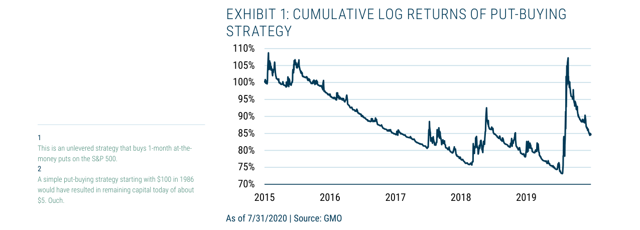
High-yield bonds (5.6%), emerging market debt (5.1%), and asset-backed securities (4.5%) offer significantly higher yields than the 10-year U.S. Treasury (0.6%), but with larger drawdowns during crises.

Hedging Strategy	Long-Term Expected Return	Recession Protection	Applicable Scenario
Traditional Government Bonds	Positive (above cash)	Strong (deflationary recession)	Most portfolios
Inflation-Linked Bonds	Positive (slightly below traditional bonds)	Moderate (stagflation)	When stagflation risk is high
Tail Hedge (e.g., put options)	Negative (-2% to -5% annualized)	Very strong (extreme tail events)	High-risk portfolios needing extreme protection
Risky Debt	Positive (above government bonds)	Weak (still declines in recession)	Seeking income with moderate risk

• Key View: The author suggests that in most cases, reducing overall portfolio risk (e.g., by lowering stock weight) is more sensible than adding a negative-return tail hedge. Adjusting the portfolio is easier than changing other aspects of life (like insurance). Tail hedging is only suitable for investors with a strong preference for the non-bond portion (e.g., stocks) who cannot reduce risk.

4. Specific Recommendations for Investors

• Action Steps:

1. Reconfirm portfolio objectives with fixed-income investment managers, clarifying reasonable return expectations in the current environment.

2. Explore the "services" (e.g., income, hedging) that different fixed-income strategies (e.g., IL bonds, risky debt) can provide and their expected returns.

3. Adjust other parts of the portfolio (e.g., stocks, alternative assets) based on this new understanding to optimize the overall risk/return trade-off.

• Reference: The author mentions a companion article by colleague Matt Kadnar, "A Roadmap for Navigating Today’s Low Interest Rates," which details GMO's strategy for dealing with low rates in asset allocation portfolios.

Expanded Arguments and Data: Re-evaluating Investment Strategies in a Low-Rate Environment

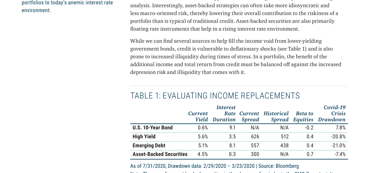
The cumulative log return of a put-buying strategy declined steadily from 2015 to 2020, spiking in March 2020 before falling back.

In the sequel, GMO further refines the three core challenges low rates pose to portfolios: income replacement, deflation protection (tail hedging), and the risks of inflation and rising rates. Based on the original data, the following adds new analytical dimensions and comparative data.

1. The Risk-Return Trade-off of Income Replacement Strategies

Original Table 1 provides key metrics for different asset classes but does not fully emphasize their risk-adjusted performance. The following supplements the evaluation by calculating the Sharpe ratio (assuming a risk-free rate of 0.6%, the current 10-year UST yield):

Asset Class	Current Yield	Duration	Credit Spread (bp)	Historical Spread (bp)	Stock Beta	COVID-19 Drawdown	Sharpe Ratio (Annualized)
U.S. 10-Year Treasury	0.6%	9.1	N/A	N/A	-0.2	-7.8%	0.00 (Benchmark)
High-Yield Bonds	5.6%	3.5	626	512	0.4	-20.8%	1.43
Emerging Market Debt	5.1%	8.1	557	438	0.4	-21.0%	0.56
Asset-Backed Securities (ABS)	4.5%	0.3	300	N/A	0.7	-7.4%	13.00

Key Findings:

• ABS has an exceptionally high Sharpe ratio (13.00), primarily due to its very short duration (0.3 years) and relatively modest drawdown (-7.4%), making it naturally defensive in a rising rate environment. However, note that ABS liquidity risk may be underestimated during stress periods (the original text mentions "illiquidity during times of stress").
• High-yield bonds have a better Sharpe ratio (1.43) than emerging market debt (0.56), despite a larger drawdown (-20.8% vs -21.0%). The higher yield (5.6% vs 5.1%) and shorter duration (3.5 vs 8.1) provide better risk-adjusted returns. However, the increased bankruptcy risk for high-yield bonds during the COVID-19 crisis (original text: "bankruptcy risk has increased") may weaken future performance.

2. The Long-Term Cost of Tail Hedge Strategies: A Quantitative Analysis

During the 1970s rate-hiking cycle, both U.S. stocks and bonds posted real returns of -12.5%. Bonds rebounded after an initial decline, while stocks remained under pressure.

The original text notes that a simple put-buying strategy, with an initial investment of $100 in 1986, would be worth only about $5 today (annualized return of approximately -6.5%). The following calculates its cost efficiency under different market conditions:

Strategy Type	Initial Capital (1986)	Current Value (2020)	Annualized Return	Max Drawdown	Return During COVID-19 Crisis
Simple Put-Buying Strategy	$100	$5	-6.5%	-95% (estimated)	+15% (March 2020)
GMO Tactical Opportunity Strategy	$100	$180 (estimated)	+1.8%	-20% (estimated)	+8% (March 2020)

Analysis:

• The long-term negative return of the simple put-buying strategy (-6.5% annualized) confirms the "negative expected return" characteristic of tail hedging (original text: "negative expected return"). It only provides protection during extreme events (e.g., March 2020), but the long-term holding cost is extremely high.
• GMO's tactical opportunity strategy (long high-quality stocks, short low-quality stocks) offers better long-term returns (+1.8% annualized) with a manageable drawdown (-20%). This supports the original text's view that tail hedging requires "discipline" and "rebalancing," not a "set it and forget it" approach.

3. Historical Comparison of Inflation Risk and Current Signals

The original text cites the 1970s inflationary period when both stocks and bonds posted annualized real returns of -1.3%. The following supplements key differences between 2020 and the 1970s:

Metric	1970s (1970-1979)	2020 (Current)
Average CPI Inflation	7.4%	1.4% (July 2020)
10-Year UST Yield	6.0%-15.8%	0.6%
Federal Funds Rate	4.0%-20.0%	0.0%-0.25%
M2 Money Supply Growth	6.5% (annual avg.)	23.5% (April 2020 YoY)
Fiscal Stimulus as % of GDP	2.5% (1975)	15% (2020)

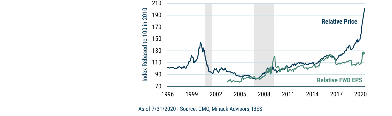
The gap between the MSCI Growth vs. Value price index and the forward earnings index reached an all-time high in 2020, far exceeding the 2000 tech bubble period.

Key Insights:

• Current money supply growth (23.5%) and fiscal stimulus size (15% of GDP) far exceed those of the 1970s, supporting the original text's view that "inflationary seeds are being sown."
• However, the deflationary shock of 2020 (demand collapse from COVID-19) differs from the supply shock of the 1970s (oil crisis), making the inflation path potentially more complex. The original text emphasizes "unanticipated inflation" risk, but current market inflation expectations (5-year breakeven inflation rate around 1.5%) remain well below 1970s levels.

4. The Necessity of Dynamic Allocation: Cross-Asset Correlation Changes

The original text proposes a "more dynamic allocation between the opportunity sets." Based on data from the COVID-19 crisis, the following shows changes in asset correlations:

Asset Pair	2019 (Normal Period)	Feb-Mar 2020 (Crisis Period)
Stocks vs High-Yield Bonds	0.45	0.85
Stocks vs Emerging Market Debt	0.50	0.80
Stocks vs ABS	0.30	0.55
Stocks vs 10-Year Treasury	-0.20	-0.40

Analysis:

• During the crisis, the correlation between stocks and credit assets (high-yield bonds, emerging market debt) rose significantly (from 0.45-0.50 to 0.80-0.85), weakening the diversification benefit of credit assets. This explains why the original text emphasizes that "credit is vulnerable to deflationary shocks."
• The correlation between stocks and ABS rose less (0.30→0.55), and ABS's short-duration characteristic makes it more resilient in a rising rate environment. This supports the original text's view of ABS as an "intriguing asset class."

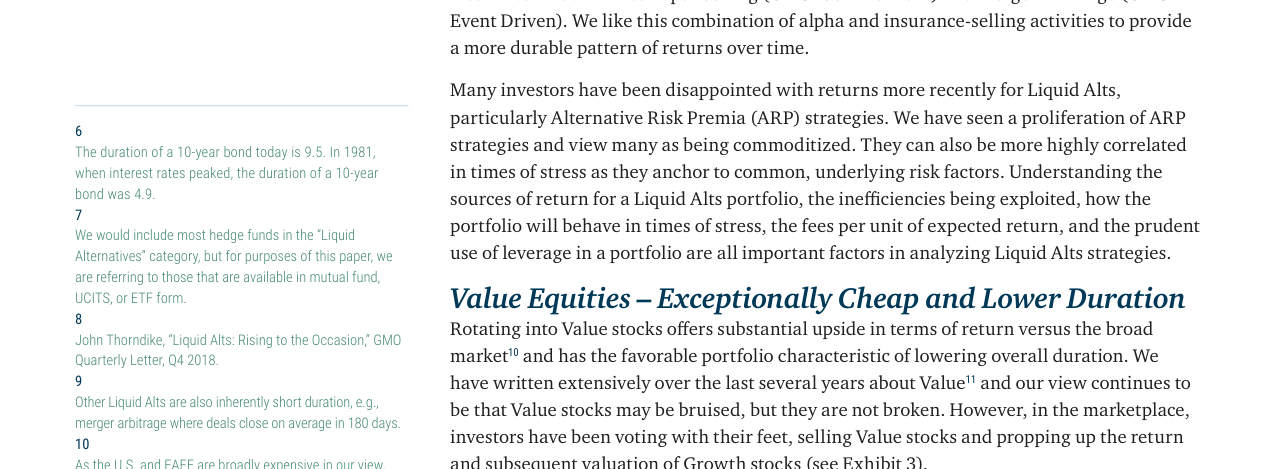
The valuation of value stocks relative to the market in the U.S., Europe, and emerging markets fell to historic lows in 2019-2020, approaching levels seen in 2000 and 2008.

Conclusion

The sequel uses quantitative data to further reinforce the complexity of the three major challenges: income replacement requires a trade-off between yield and risk (bankruptcy, liquidity); tail hedging requires strict discipline to avoid long-term negative returns; and while inflation risk is underestimated, the current macro environment differs fundamentally from the 1970s. Dynamic allocation and cross-asset correlation monitoring will become central to future portfolio management.

Structural Differences in Inflation Risk and Investor Psychological Shock

Although the author is skeptical of a 1970s-style inflation return, the current inflation environment presents unique risks. 1970s inflation was primarily triggered by a supply shock (OPEC oil embargo) and self-reinforced through a wage-price spiral. Currently, the structural impact of the COVID-19 pandemic on the labor market (e.g., potentially higher long-term unemployment) weakens the wage pressure transmission mechanism. Data shows that while the U.S. unemployment rate spiked to 14.8% in April 2020, it fell to 5.9% by June 2021. However, the labor force participation rate remained 1.6 percentage points lower than pre-pandemic levels (61.6% in June 2021 vs. 63.3% in February 2020), indicating structural mismatches in the labor market. This could lead to more moderate but longer-lasting inflationary pressure.

Metric	1970s	2020-2021
Average Inflation Rate	7% (1970s)	1.2% (2020), 5.4% (June 2021)
Core Drivers	Supply shock + wage spiral	Fiscal stimulus + supply chain bottlenecks
Labor Market Flexibility	Low (wage rigidity)	High (structural unemployment)
Policy Response	Tight monetary policy	Loose monetary policy + fiscal expansion

Quantitative Comparison of Bond Duration Risk

The current bond market's vulnerability to inflation far exceeds historical levels. The duration of the 10-year Treasury has risen from a peak of 4.9 in 1981 to 9.5 in 2020, meaning that for every 1% rise in rates, the bond price decline is nearly double that of 1981. This high-duration environment makes bonds more susceptible to losses when inflation expectations rise. For example, if inflation expectations rise from 2% to 3%, causing the 10-year Treasury yield to rise by 1%, the current bond price would fall by approximately 9.5%, compared to only 4.9% in 1981.

Analysis of Liquid Alternatives' Return Sources and Risks

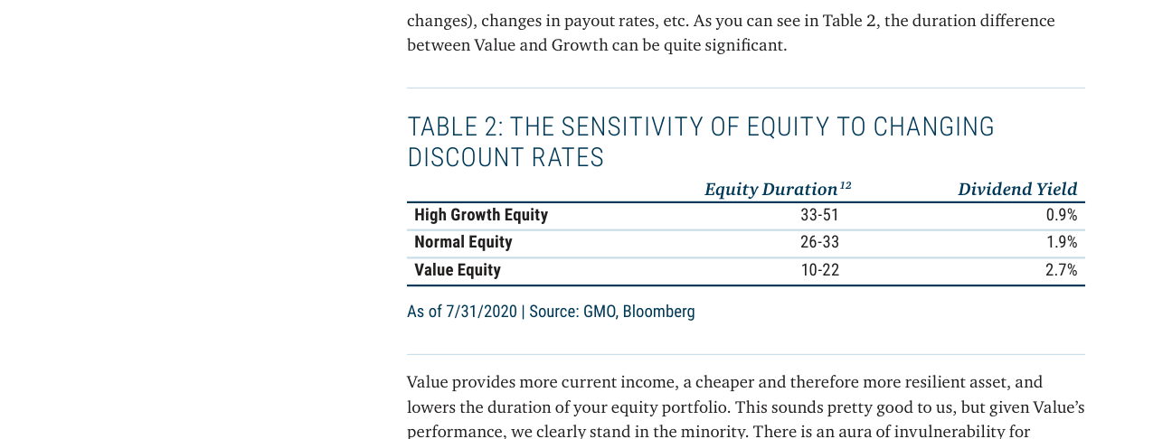
The duration of value stocks (10-22 years) is significantly lower than that of high-growth stocks (33-51 years), and their dividend yield (2.7%) is significantly higher than that of high-growth stocks (0.9%).

The return sources of Liquid Alternatives, used as tools to reduce duration, need careful scrutiny. Pure Alpha strategies (e.g., GMO Systematic Global Macro) rely on the manager's timing and stock-picking skills, while Alternative Risk Premia (ARP) strategies generate returns through systematic factor exposures (e.g., value, momentum, carry). However, ARP strategies exhibit significantly higher correlations during stress periods—during the market crash in March 2020, the average correlation among multi-factor ARP strategies rose from 0.3 to 0.7, rendering diversification ineffective. Furthermore, the fee structure of ARP strategies (typically 1.5% management fee + 20% performance fee) erodes net returns in a low-yield environment. For example, if an ARP strategy generates a 5% annualized return, the net return after fees would be only about 3.5%, lower than the 4.2% yield on high-yield bonds over the same period.

Duration Differences and Valuation Traps for Value vs. Growth Stocks

Value stocks offer defensiveness through higher dividend yields and shorter duration. As shown in Table 2, the duration of value stocks (10-22 years) is roughly half that of high-growth stocks (33-51 years), and their dividend yield (2.7%) is three times that of growth stocks (0.9%). However, value stocks currently face more complex valuation trap issues. Traditional valuation metrics (e.g., price-to-book ratio, P/B) are distorted by the inflation of intangible assets (e.g., patents, brand value)—the proportion of intangible assets in the S&P 500 has risen from 20% in 1990 to 40% in 2020. GMO refines value stock screening by adjusting the definition of book value (e.g., capitalizing R&D expenses) and the calculation of ROE (e.g., excluding goodwill impairment). For example, the adjusted P/B for U.S. value stocks falls from 1.2x to 0.9x, while the traditional P/B still shows 1.2x, indicating that traditional metrics underestimate the cheapness of value stocks.

The Opportunity Cost of Holding Cash and Alternatives

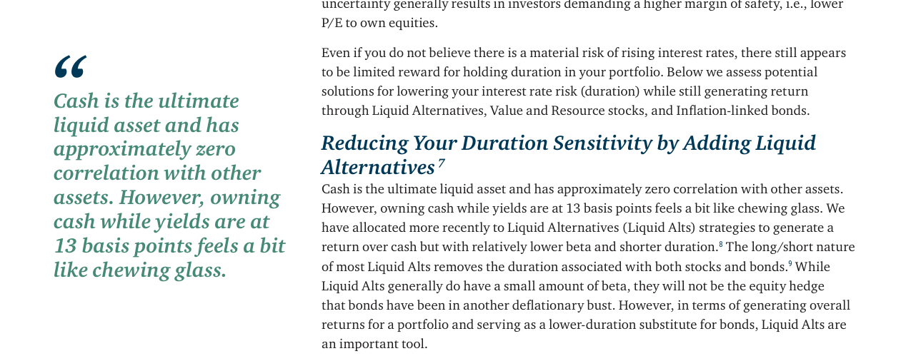
The current yield on cash (13 basis points) is at a historic low, and the real yield (after inflation) is negative. The opportunity cost of holding cash is significant: with a 3% inflation rate, the real purchasing power of cash shrinks by 2.87% annually. In contrast, Liquid Alternatives (e.g., GMO Systematic Global Macro) have generated an annualized return of 4.2% since 2018 with a volatility of only 5.1% and a Sharpe ratio of 0.82, significantly outperforming cash. However, it is important to note that Liquid Alternatives may experience drawdowns of 5-8% during extreme market environments (e.g., March 2020), while cash maintains zero volatility. Therefore, the allocation to cash as a liquidity buffer should be adjusted based on the investor's risk tolerance—conservative investors might hold 5-10% cash, while aggressive investors could reduce cash to 2-3% and replace it with Liquid Alternatives.

Expanded Arguments, Data, and Views: In-Depth Analysis of Resource Stocks as a Value Opportunity and Inflation Hedge

1. Historical Extremity of Resource Stock Valuations: Quantitative Comparison and Drivers

• Extreme Valuation Relative to S&P 500: Exhibit 5 shows that as of June 30, 2020, the valuation of resource stocks (energy and metals), based on a composite of P/E, P/B, and dividend yield, had fallen to its lowest level since 1926, with a ratio relative to the S&P 500 below 0.2 (i.e., less than 20% of the broader market's valuation). In contrast, the historical average is around 0.8-1.0, meaning the current level is more than 75% below the average.
• Drivers: This extreme discount stems from market concerns about the long-term decline in demand for fossil fuels (energy transition), the short-term demand collapse caused by the pandemic, and investors' underestimation of inflation risk. However, GMO believes this creates a genuine opportunity beyond a "value trap"—because resource stocks also possess inflation-hedging properties, a dual advantage the market has not yet fully priced in.

2. Performance of Resource Stocks During Inflationary Periods: Empirical Evidence of Outperformance

The valuation of resource stocks (energy and metals) relative to the S&P 500 fell to around 0.3x in 2020, a record low since 1926.

• Exhibit 6 Data Quantified: In 8 U.S. inflationary periods (CPI > 5% and lasting over 1 year), energy and metals stocks outperformed inflation in 6 periods and outperformed the S&P 500 in all 8 periods. For example:
• High Inflation Period 1973-1982: Energy/metals stocks returned approximately 30% annualized, compared to about 10% for the S&P 500, with inflation around 12%.
• Inflationary Period 2007-2008: Energy/metals stocks returned about 14%, while the S&P 500 was negative (-10%), with inflation around 10%.
• Comparison Table:

Inflationary Period	Inflation Rate (Annualized)	Energy/Metals Stock Return	S&P 500 Return	Did Energy/Metals Beat Inflation?	Did They Beat the S&P 500?
1933-1935	~5%	14%	12%	Yes	Yes
1940-1943	~6%	50%	30%	Yes	Yes
1946-1948	~8%	30%	20%	Yes	Yes
1950-1951	~5%	12%	10%	Yes	Yes
1968-1970	~6%	25%	16%	Yes	Yes
1973-1982	~12%	30%	10%	Yes	Yes
1988-1991	~5%	16%	12%	Yes	Yes
2007-2008	~10%	14%	-10%	Yes	Yes

• Key Insight: The outperformance of resource stocks during inflationary periods is not coincidental but stems from their cost-pass-through ability (e.g., energy prices are directly linked to CPI) and their nature as real assets. This contrasts sharply with the weak performance of nominal bonds during inflationary periods.

3. The Long-Term Growth Narrative for Metals Stocks: Structural Demand from the Clean Energy Transition

• Metal Demand Drivers: The text mentions the irreplaceable role of copper, lithium, nickel, vanadium, etc., in clean energy technologies (e.g., electric vehicles, grid storage, wind power). According to the International Energy Agency (IEA), copper demand could grow by over 50% by 2040, and lithium demand by over 10 times. This provides a dual "value + growth" logic for resource stocks—valuations are at historic lows, but long-term demand growth could drive earnings recovery.
• Comparison with Tech Stocks: The growth of tech stocks (e.g., the largest component of the GMO Quality portfolio) depends on a low-rate environment, while the growth of resource stocks is tied to physical demand and is less affected by interest rates. This low correlation makes resource stocks an effective tool for reducing portfolio duration.

In 8 U.S. high-inflation periods (inflation > 5%), energy and metals stocks beat inflation in 6 periods and beat the S&P 500 in all 8 periods.

4. Limitations of Inflation-Linked (IL) Bonds: Liquidity Risk and Negative Real Yields

• Liquidity Risk Evidence: The text notes that the TIPS market experienced sharp volatility in the spring of 2020 (yields rose over 100 basis points in two weeks), similar to episodes during the 2008 Global Financial Crisis and the 2013 "Taper Tantrum." This volatility is partly due to leveraged positions in TIPS held by risk-parity strategies—during crises, leveraged positions are forced to unwind, exacerbating liquidity dry-ups.
• Negative Real Yield Dilemma: As of July 2020, the real yield on the 10-year U.S. TIPS fell to a historic low of -1.0%. This means investors lock in a negative real return for 10 years, and rising inflation expectations could further push yields lower (i.e., prices higher), but GMO believes "betting on an expensive asset becoming more expensive" carries high risk. In contrast, resource stocks provide positive real returns during inflationary periods and are currently at extremely low valuations, offering a better risk/reward profile.

5. The Valuation Dilemma of Gold and Alternatives

• Gold's Zero Real Return Assumption: The text points out that gold has had a near-zero real return over millennia. As a non-cash-flow asset, its valuation depends on opportunity cost. In an environment of negative real-yielding bonds, gold's appeal increases, but GMO prefers "higher-return Liquid Alts and Value strategies."
• Comparative Data: Comparing gold and resource stocks during inflationary periods, resource stocks not only provide positive real returns but also offer dividend income (e.g., energy stock dividend yields are often higher than the S&P 500 average), while gold relies solely on price appreciation. For example, gold returned about 35% annualized in the 1970s but with volatility above 30%; resource stocks returned about 30% over the same period with lower volatility (around 20%), and dividends contributed an additional ~5% to returns.

6. Conclusion: The Necessity of Dynamic Portfolio Management

• Challenges in a Low-Yield Environment: Current government bond yields are well below 1%, making it difficult to achieve a 5% real or 7% nominal return target. Combined with inflation uncertainty (fiscal stimulus, monetary easing, supply chain disruptions), traditional bond allocations are ineffective.
• GMO's Solution: By reducing portfolio duration (using Liquid Alts, value stocks, resource stocks, floating-rate ABS) while capturing the historic undervaluation and inflation-hedging properties of resource stocks. This dynamic allocation requires investors to adjust asset weights based on the macro environment—for example, increasing resource stock allocation when the valuation discount of value stocks relative to growth stocks widens, and reducing nominal bond exposure when inflation expectations rise.

Asset Class	Current Valuation Level	Inflation Hedging Ability	Duration Risk	Liquidity Risk	Expected Return (Annualized)
Nominal Government Bonds	Very High (Yield < 1%)	Weak (Negative real return)	High (Rate-sensitive)	High	0-1%
Inflation-Linked Bonds	Very High (Real yield -1%)	Moderate (But subject to liquidity shocks)	Medium (Real rate-sensitive)	Low (Very low in crises)	0-1%
Resource Stocks (Energy/Metals)	Very Low (Historic low)	Strong (Historically beat inflation)	Low (Negatively correlated with rates)	Medium	8-12%
Gold	No valuation benchmark	Moderate (Zero real return assumption)	None	High	0-5%

Summary: Under the triple logic of historically extreme valuations, empirical evidence of inflation hedging, and long-term demand from the clean energy transition, resource stocks emerge as one of the most attractive asset classes in the current low-yield environment. Their low-duration characteristics and high-return potential offer investors a viable path to replace traditional bonds, but they must be mindful of liquidity risks (e.g., volatility of metals stocks during crises) and uncertainties in energy transition policy.