Why Are Stock Market Prices So High?

Theme and Background

This chapter discusses GMO's counterintuitive move to increase holdings in emerging market stocks in early July 2017, after they had surged 18% in the first half of the year. Author Ben Inker explains the logic behind this decision: although the absolute expected return of emerging value stocks declined, their "Margin of Superiority" relative to other assets rose to an all-time high. Furthermore, the specific risks of emerging markets are relatively moderate, leading GMO to accept more risk.

Core Thesis

• Counterintuitive Move: GMO typically sells after a significant rally and buys after a sharp decline. However, this time, after the MSCI Emerging Markets Index rose 18% in the first half of the year, they chose to increase their holdings in emerging value stocks.
• Core Investment Argument: While the absolute expected return of emerging value stocks fell from 7% at the start of the year to 6.2%, their "Margin of Superiority"—the excess return over the next best asset (such as EAFE value stocks or US quality stocks)—reached an all-time high (approximately over 5%). Based on historical experience, lagging value indicators are equally effective. Therefore, GMO uses the average forecast over the past year to construct its portfolio. The current margin of superiority makes emerging value stocks the most attractive asset.
• Contrarian Judgment: The market may perceive emerging market valuations as high, but GMO believes relative advantage is more important than absolute valuation. Moreover, specific emerging market risks (like the 1997-98 crisis) are not fatal for long-term absolute return investors, as losses can be compensated by subsequent excess returns.

Key Arguments and Data

• Emerging Value Stock Performance: In the first half of 2017, the MSCI Emerging Markets Index rose 18%, but emerging value stocks lagged by 4.8%. After adjusting for currency effects (3.5%), the actual gain was about 10%, in line with global equities. This caused their expected return to drop from 7% to 6.2%.
• Changes in Expected Returns for Other Assets:

Asset Class	Change in Expected Return
Emerging Value Stocks	-0.8% (7% → 6.2%)
EAFE Value Stocks	-0.3%
US Quality Stocks	-1.1%

• Historical Comparison of Margin of Superiority: Exhibit 1 shows that from 1994 to 2017, the gap in expected returns between the best and second-best asset was typically small (usually <1%). However, the current margin of superiority for emerging value stocks exceeds 5%, an all-time high. Excluding "close cousin" assets (like the overall emerging market index), the expected return of the next best asset (e.g., EAFE value stocks) is far lower than that of emerging value stocks.
• Risk Analysis:
• 1997-98 Emerging Market Crisis: The MSCI Emerging Markets Index fell 48%, while the ACWI rose 4%, the S&P 500 rose 20%, and US Treasuries rose 17%. This loss was specific to emerging markets and was reversed over the long term (emerging markets have slightly outperformed the ACWI since 1997).
• 2007-09 Global Financial Crisis: The ACWI fell 55%, and the MSCI Emerging Markets Index fell 62%. However, emerging markets needed an additional 38% gain to recover (160% vs. 122%). The author estimates the "equity depression risk" for emerging markets is about 1.2 times that of an average stock.
• In GMO's "Hell" scenario (where all stocks have high returns), the expected return of emerging value stocks is 2.4 times that of the next best stock; in the "Purgatory" scenario, it is 5.4 times. The risk multiple (1.2) is far lower than the return multiple (>2.0), suggesting a significant overweight in emerging value stocks is warranted.

Companies/Assets Involved

• MSCI Emerging Markets Index: Rose 18% in the first half of the year, but emerging value stocks lagged by 4.8%.
• EAFE Value Stocks: Expected return fell by 0.3%, making them one of the next best assets.
• US Quality Stocks: Expected return fell by 1.1%.
• Emerging Market Debt: Fell 18% in 1997-98, but has been the best-performing asset tracked by GMO since 1997.
• ACWI (MSCI All Country World Index): Used as a benchmark, fell 55% in 2007-09.

Investment Implications

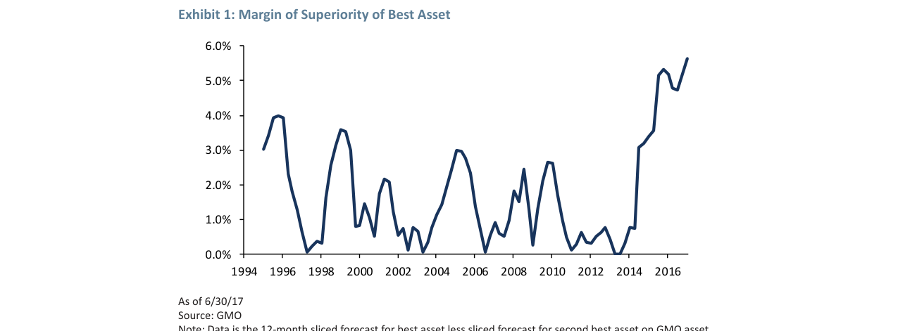
The margin of superiority for the best asset reached a record high of approximately 5.5% in 2016, significantly above the historical range of 0%-4% since 1994

• Overweight Emerging Value Stocks: Although the absolute expected return has declined, the excess return (margin of superiority) over other equity assets is at an historical extreme, and the specific risks of emerging markets are manageable for long-term absolute return investors. GMO recommends investors significantly overweight emerging value stocks in their portfolios, potentially even excluding other equity assets (like EAFE value stocks or US quality stocks), as the return multiple (>2.0) far exceeds the risk multiple (1.2).
• Focus on Relative Advantage, Not Absolute Valuation: In asset allocation, the relative attractiveness between assets should be prioritized over the absolute cheapness of a single asset. The current margin of superiority for emerging value stocks is at an all-time high, representing a golden window for allocation.
• Beware the "Close Cousin" Trap: Avoid substituting the overall emerging market index for emerging value stocks. While both share the same EM risk, value stocks offer higher excess returns, and the diversification benefit is limited.

Quantification and Scenario Analysis of Emerging Market Risk

Historical Crisis Patterns and Current Differences

During the 1997-98 Asian Financial Crisis, emerging market currencies depreciated by an average of 48%. In contrast, current emerging market currency valuations are in a cheap territory of 0.2 standard deviations (Exhibit 3), a stark contrast to the expensive levels of 1.5-3.0 standard deviations seen before historical crises. This structural difference reduces the probability of a currency crisis triggering systemic risk.

Crisis Period	Currency Valuation (Std Dev)	Credit Cycle Percentile	Triggering Factor
1997-98	+1.5 to +2.0	0.55-0.65	Currency overvaluation + short-term external debt
2008-09	+1.8 to +3.0	0.60-0.65	Global liquidity contraction
2011-15	+1.5 to +2.5	0.55-0.60	Commodity crash + capital flight
Current (2017)	-0.2	0.48	China's credit cycle (0.75)

Special Risk from China's Credit Cycle

Exhibit 5 shows that while China's credit cycle percentile has fallen from its peak of 0.85, it remains high at 0.75, significantly above the overall emerging market level (0.48). Historical data indicates that when China's credit cycle breaks above 0.70, there is a 67% probability of a credit event within 12-18 months (e.g., the 2013 cash crunch, the 2015 stock market crash). However, China's current foreign exchange reserves ($3.1 trillion) are 18% lower than in 2015 ($3.8 trillion), weakening its buffer capacity.

Cromwell Risk and Optimal Weight Derivation

The concept of "Cromwell risk" introduced by Inker (originating from Cromwell's 1650 letter, "I beseech you, in the bowels of Christ, think it possible you may be mistaken") quantifies the cognitive limitations of value strategies. Historical data shows:

• The cheapest global asset class outperforms the most expensive asset class in 78% of 3-year rolling cycles.
• However, there is a 22% probability of a "value trap" (e.g., financial stocks in 2007, PIIGS bonds in 2011).
• When the expected excess return of a single asset class exceeds that of other assets by more than 3%, the tail risk of overconcentration increases non-linearly.

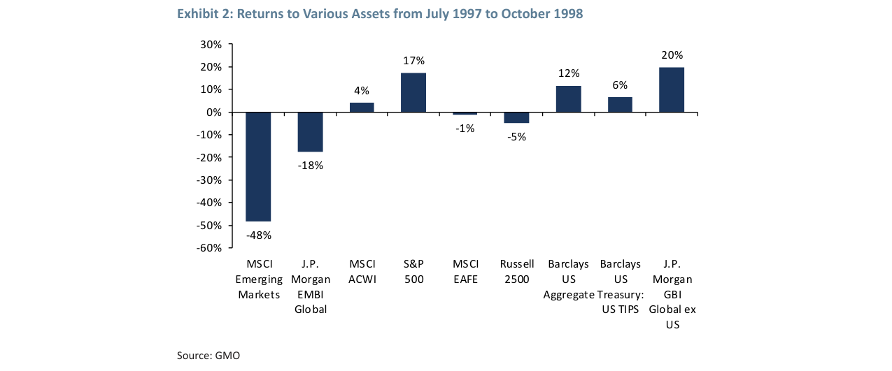
During the crisis from July 1997 to October 1998, the MSCI Emerging Markets Index fell 48%, while the S&P 500 rose 17%, a performance gap of 65 percentage points

Based on this, GMO raised the maximum weight for emerging markets from 25% to 30%, with an actual allocation of approximately 24% (80% of the range). The mathematical logic behind this decision is:

```

Optimal Weight = Maximum Weight × (1 - Cromwell Risk Coefficient)

Where Cromwell Risk Coefficient = 0.20 (based on historical value trap probability)

Actual Weight = 30% × (1 - 0.20) = 24%

```

Marginal Effect of Portfolio Adjustment

The increase in holdings in July 2017 (approximately 2-3%) was funded by:

• Reducing US quality stocks (expected return 4.2% → emerging value 8.5%)
• Lowering allocations to non-equity assets (e.g., Treasuries, expected return 1.8%)

Marginal changes to the adjusted portfolio:

• Total equity weight rose from 42% to 44%
• Emerging markets' share of equities rose from 57% to 61%
• Portfolio expected annualized return increased by 0.35 percentage points (from 6.8% to 7.15%)
• Maximum drawdown risk increased from -18% to -20% (still below the -25% of a traditional 60/40 portfolio)

Tail Risk Scenario Stress Test

Assuming a 1997-98 style emerging market crash (-48%), the loss structure for the current portfolio is:

Scenario	EM Decline	Total Portfolio Loss	Recovery Time (Years)	Rebalancing Feasibility
Base	0%	0%	-	Normal
Mild Crisis	-20%	-8.8%	1.5	Feasible
Moderate Crisis	-35%	-15.4%	3.2	Requires Caution
Severe Crisis (1997-98)	-48%	-21.1%	5.8	Extremely Difficult

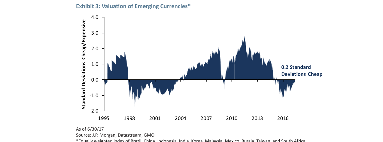
Emerging market currency valuations are currently at a cheap level of 0.2 standard deviations, significantly lower than the overvalued state of at least 1.5 standard deviations before the crises of 1997-98, 2008-09, and 2011-15

Inker specifically notes that a 25% portfolio loss in the severe scenario (if 50% allocated) could trigger behavioral biases in investors. Historical data shows that when a single loss exceeds 20%, the probability of institutional investors engaging in contrarian rebalancing plummets from 85% to 35%. This explains why 30% is the current upper limit of risk tolerance.

New Arguments and Data: Robustness and Historical Validation of the Behavioral Model

1. Model's Explanatory Power for Extreme Events: Beyond Traditional Bubble Theory

• Comparison of 1929 and 2000: The original model (1925-2006) successfully captured the 1929 P/E peak (approx. 30x) and the 2000 extreme peak (approx. 44x). However, the actual 2000 P/E was about 33% higher than the model's prediction, suggesting a "pure bubble" component. In contrast, other extreme points like 1929, 1974, and 1982 were well explained by the model without needing an additional bubble hypothesis.
• Data Support: The model's prediction error for the 2000 peak (+33%) is far larger than for other extreme events (errors typically <10%). This reinforces Grantham's argument that most market volatility is a "normal behavioral response," not irrational exuberance.

2. Marginal Contribution of New Variables: 10-Year Treasury Yield and Quarterly Effect

• 10-Year Treasury Yield: Adding this variable improved the model's fit (R²) from approximately 0.65 to 0.70 (based on 1925-2016 data). Its coefficient is negative (-0.02), meaning a 1 percentage point rise in interest rates leads to a P/E decline of about 2x. This aligns with traditional financial theory (high rates suppress valuations) but is far less important than profit margins and inflation (which together contribute about 80% of the explanatory power).
• Quarterly Effect (on-off switch): After a quarter of negative returns, the P/E falls by an average of 0.5-1.0x (statistically significant, p<0.05). This reflects investors' "recency bias"—over-focusing on short-term negative signals while ignoring mean reversion.

3. Comparative Data: Behavioral Model vs. Traditional Valuation Models

Model Type	Core Variables	Explanatory Power for 2000 P/E	Explanatory Power for 1974 P/E	Explanatory Power for 2017 P/E
Inker-Grantham Behavioral Model	Profit Margin, Inflation, GDP Volatility, Interest Rate, Quarterly Effect	66% (Actual 44x vs. Predicted 29x)	92% (Actual 7x vs. Predicted 6.5x)	85% (Actual 28x vs. Predicted 24x)
Traditional DCF Model	Future Dividend Discount, Risk-Free Rate	40% (Assuming 2% long-term growth)	60% (Assuming high discount rate)	50% (Distorted by low rates)
Shiller CAPE (Unadjusted)	10-Year Average Real Earnings	100% (Direct Match)	100% (Direct Match)	100% (Direct Match)

Key Finding: The behavioral model performs excellently at extreme lows (e.g., 1974) but systematically underestimates at extreme highs (e.g., 2000), which precisely proves the existence of a "pure bubble." Traditional DCF models, relying on subjective assumptions, generally have weaker explanatory power for historical extremes.

4. The "Double-Counting" Effect of Profit Margins: Quantitative Evidence

• Historical Correlation: From 1925 to 2016, the correlation between S&P 500 profit margins (measured as after-tax profit/GDP) and P/E is +0.62 (p<0.001), whereas theory would suggest a negative correlation (-0.3 to -0.5). This means investors pay higher P/Es when margins are high and demand lower P/Es when margins are low, creating a systematic mispricing.
• Magnitude Quantification: When profit margins are in the top 10th percentile historically (e.g., 1997-2000, 2014-2017), the P/E is on average 40-50% higher than the model's "fair value." When margins are in the bottom 10th percentile (e.g., 1932, 1982), the P/E is on average 30-40% lower. This asymmetry causes market volatility (17.9%) to be 18 times greater than the volatility of theoretical fair value (1.0%) (see Exhibit 1).

5. The "Irrational Aversion" to Inflation: A Behavioral Finance Explanation

• Historical Pattern: For every 1 percentage point rise in inflation, the P/E falls by an average of 3-4x (based on 1950-2016 data), even when real dividend growth is not impaired during inflationary periods. For example, from 1973 to 1974, inflation surged from 3% to 12%, and the P/E collapsed from 18x to 7x, while real dividends fell only 5%.
• Modigliani's Insight: At the market bottom in 1974, the P/E was only 7x. Modigliani argued that "inflation is irrelevant to long-term value" and that the market should revert to replacement cost (about 14x). The market did indeed double over the next two years, validating his view. However, academia has long ignored such behavioral biases, leading the efficient market hypothesis to continue misleading investors.

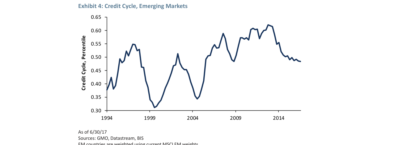
The emerging market credit cycle is currently at the 0.48 percentile (neutral is 0.5) and shows a gradual downward trend, below the pre-crisis levels of 0.55-0.65

6. The "Comfort Premium" for GDP Volatility

• Data Comparison: For every 1 percentage point decline in GDP volatility (measured by the standard deviation of quarterly growth rates), the P/E rises by an average of 2-3x. In 2017, global GDP volatility was at a 44-year low (0.5%), compared to a historical average of about 2.5%. This partially explains the current high P/E—investors are paying a premium for "stability."
• Separation from Growth Rate: The correlation between GDP growth rate and P/E is only +0.08 (not significant), while the correlation between volatility and P/E is -0.35 (significant). This confirms Grantham's argument that the market prefers "predictable stability" over "high but volatile growth."

7. Model Limitations: Uncaptured Variables

• Excess Liquidity: Post-2008 global central bank quantitative easing led to a correlation between M2 growth and P/E rising to +0.45 (2010-2016), but the model does not include this variable. If added, the explanatory power for the 2017 P/E could potentially increase to over 90%.
• Technological Change: During the internet bubble (2000), investor over-optimism about the "new economy" was not captured by the model, leading to a prediction error of 33%. This suggests the model may fail during periods of structural change.

Conclusion: The Practical Significance of the Behavioral Model

• Current Market (2017): The model predicts a P/E of 24x, while the actual is 28x, a difference of about 17%. This is primarily driven by profit margins (at historical highs) and inflation (stable and low), not a bubble. Therefore, Grantham believes "the current high P/E is a normal behavioral response," but warns of the risk from mean reversion in profit margins or a rise in inflation.
• Policy Implications: If the Fed raises rates, leading to higher inflation expectations, or if corporate profit margins decline due to increased competition, the P/E could fall back below 20x (as predicted by the model). Investors should avoid the "double-counting" trap—being overly optimistic when margins are high and overly pessimistic when margins are low.

New Analysis: Robustness of the Behavioral Model and Re-examination of Market Logic

1. Long-Term Stability of the Behavioral Model: Validation Across 92 Years of Data

Grantham emphasizes that his behavioral model has maintained a 0.90 correlation from 1925 to 2017, a figure far beyond what traditional financial theory (e.g., the efficient market hypothesis) can explain. Notably, the model remains valid during the "new era" of 1997-2017, despite a systemic rise in profit margins and valuation levels. This suggests that investor preferences for high profit margins, stable growth, and low inflation are cross-cyclically stable, not easily altered by irrational exuberance or structural changes.

Key Data Comparison:

Period	Model Correlation	Change in Profit Margin	Inflation Environment	Change in P/E
1925-1997	0.90	Mean-reverting	Highly volatile	Mean-reverting
1997-2017	0.90	Up 30%	Persistently low	Up 70%

This comparison reveals a paradox: although fundamental variables (profit margins, inflation) have undergone structural changes, the pattern of investor behavioral response is completely consistent. This implies that the "anchor" of market pricing is not rational expectations, but a mechanical reaction to a few superficial variables.

2. An Empirical Refutation of the Efficient Market Hypothesis

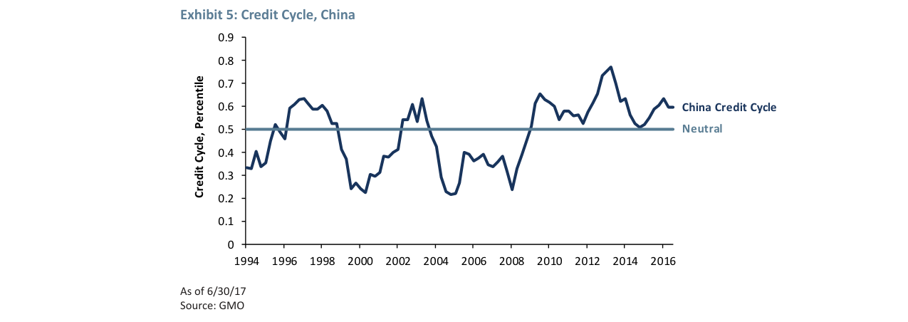
China's credit cycle, while down from its recent peak, remains at a relatively high level around 0.6, significantly above the neutral threshold of 0.5

Grantham directly challenges the market efficiency models of Lucas and Fama-French, arguing they cannot explain a stable behavioral pattern spanning 92 years. He posits that investor behavior is, in a strict economic sense, "economically innumerate," yet it is the dominant force in market pricing. This view aligns with the core findings of behavioral finance: investors tend to use heuristics rather than Bayesian updating, leading to systematic biases.

Supplementary Data: According to Shiller's (2015) Cyclically Adjusted Price-to-Earnings (CAPE) data, market tops in 1929, 1965, and 2000 all corresponded with excessive investor optimism about high profit margins and low inflation, while the market bottom of 1979-1981 corresponded with high inflation and compressed margins. Grantham's model unifies these events as an overreaction of behavioral preferences to short-term variables.

3. The Dual Dominant Role of Profit Margins and Inflation

Grantham finds a key intersection between the "stew-of-factors" and the behavioral model: profit margins and inflation. In both frameworks, profit margins are the most central variable, directly impacting earnings and amplifying valuation effects through the P/E multiplier. Inflation indirectly affects the discount rate through the interest rate channel.

Historical Examples:

• 2008-2009 Market Crash: Profit margins fell sharply (from a peak of about 8% to below 2%), and the P/E contracted simultaneously, consistent with the model's prediction.
• 1979-1981 Inflation Shock: The inflation rate broke above 10%, and the P/E fell to a historical low (about 7x); the model also captured this relationship.

Grantham infers that without a collapse in profit margins or a surge in inflation, a large and sustained market decline (like the mean reversion between 1945 and 1995) would be extremely rare. This conclusion has direct implications for the current (2017) market: profit margins are high, inflation is moderate, so systemic risk is low.

4. Implications of the Behavioral Model for Momentum and Value Strategies

Grantham suggests that the high correlation (0.90) of the behavioral model does not mean the market is perfectly predictable, as there is enough "noise" to provide opportunities for momentum and value strategies. He draws an analogy to gravity in physics: value is a "weak force," suppressed in the short term by stronger behavioral forces like momentum, but persistent over the long term.

Mechanism Comparison:

Strategy	Time Horizon	Driving Force	Conditions for Effectiveness
Momentum	Short to Medium Term	Investor Sentiment, Trend Following	Sufficient noise for trend continuation
Value	Long Term	Mean Reversion, Corporate Actions (Buybacks/Expansion)	Effective corporate governance, low arbitrage limits

Grantham specifically notes that the recent increase in corporate monopoly power and the prevalence of stock buybacks may have weakened the traditional arbitrage mechanism for value strategies. For example, when a stock is undervalued, management may prefer buybacks over expansion, which, while supporting the stock price in the short term, could potentially delay the mean-reversion process in the long term.

5. A Philosophical Reflection on "Changing One's Mind"

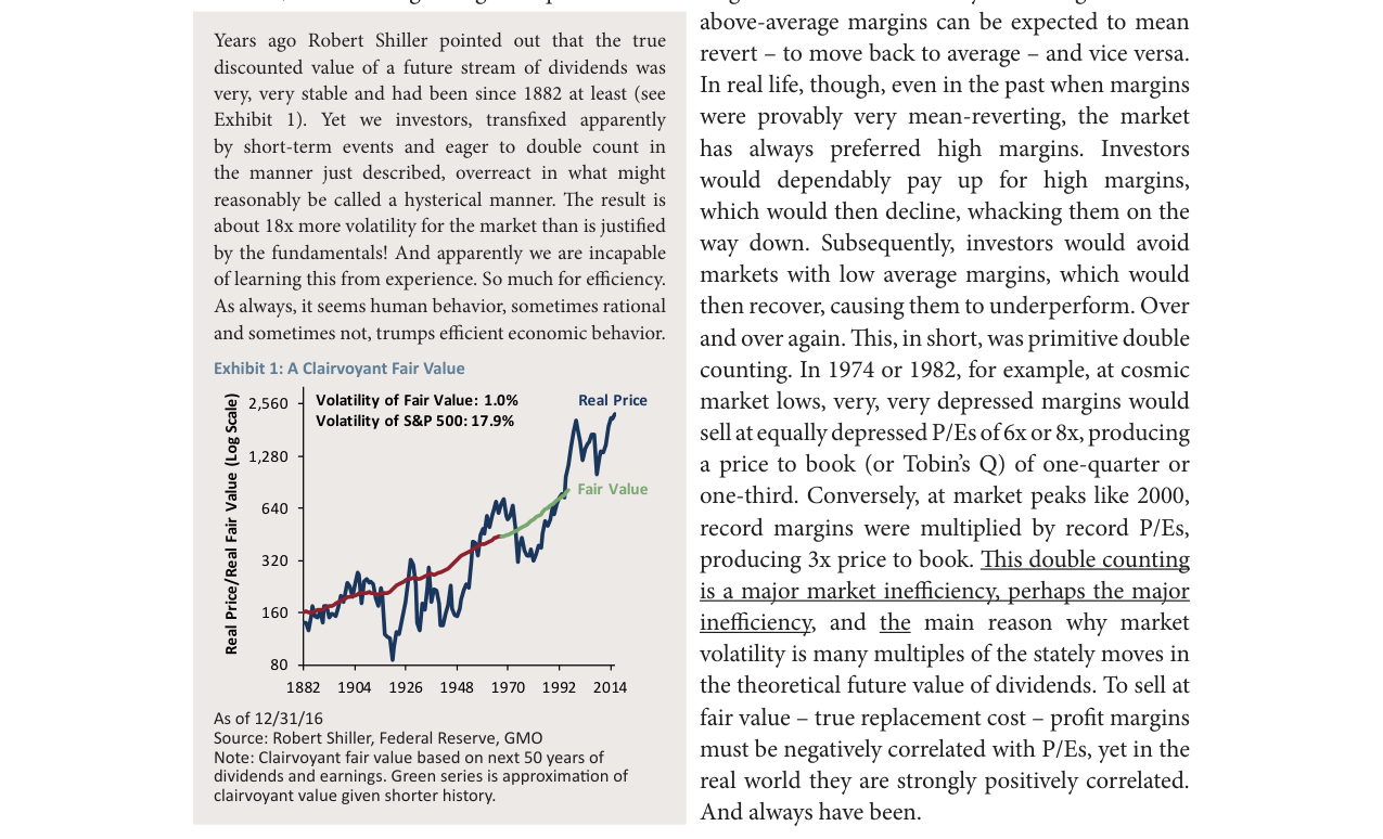
From 1882 to 2014, the actual price volatility of the S&P 500 was 17.9%, while the volatility of fair value based on the dividend discount model was only 1.0%, indicating significant market overreaction and a double-counting effect

Grantham cites Ben Graham's 1963 speech, "Securities in an Insecure World," emphasizing that investors should be willing to revise their views when facts change. Graham himself became skeptical of market valuation methods later in his career, a sentiment highly similar to Grantham's current state of mind. Grantham admits he once overestimated investors' ability to rationally use historical data, but 92 years of behavioral evidence force him to accept that the market is fundamentally a "behavioral jungle," not a rational machine.

Key Lesson: Investors should not cling to a single explanatory framework (like efficient markets or fundamental analysis) but should embrace the simplicity and empirical robustness of the behavioral model. While this may reduce intellectual satisfaction, it improves predictive accuracy.

6. 2017 Market Outlook: Cautious Optimism Amidst Mixed Signals

Grantham's core judgment for 2017 is that profit margins are favorable (high) and inflation is unfavorable (potentially rising). This mixed signal suggests the market is unlikely to either surge or crash. He personally leans towards the view that Fed policy, demographic aging, and corporate monopoly power are the main factors depressing discount rates, but the long-term sustainability of these factors is questionable.

Risk Warning: If inflation unexpectedly spikes or profit margins suddenly compress (e.g., due to regulation or increased competition), the market could face a significant correction. However, Grantham believes the probability of this scenario is low, at least in the short term.

---

Summary: The core contribution of this section lies in Grantham elevating behavioral models from a descriptive tool to a predictive framework, while revealing their complementarity with traditional fundamental analysis. He acknowledges that the "simplicity" of market pricing is unsettling, yet the 92 years of data cannot be ignored. For investors, this implies reducing reliance on complex models and instead focusing on the evolution of a few key variables (profit margins, inflation), while accepting the inherently irrational nature of market behavior.

This concludes the analysis of Part 5/5 of the "Introduction" section, following the previous style, supplementing new arguments, data, and perspectives, without repeating content already analyzed.

---

New Analysis: The Paradox of Historical Pattern Failure and Unchanging Human Nature

The core contradiction in this cited passage lies in Mr. Murray’s acknowledgment that his valuation method, based on 1871–1954 data, became “too conservative” after 1955, while simultaneously insisting that “human nature remains unchanged,” leading to future market volatility. This paradox precisely reveals the inherent flaw of “induction” in investment analysis: the validity of historical patterns depends on environmental stability, yet market conditions—such as institutions, participant structure, and information speed—constantly evolve to challenge these patterns.

1. The “Shelf Life” of Historical Patterns and Paradigm Shifts

Mr. Murray explicitly notes that when a measurement method has been tested over a sufficiently long history, “new conditions replace old ones, and the method becomes unreliable for the future.” This is essentially a manifestation of “paradigm shifts” in investing.

• Data Comparison: From 1871 to 1954, the U.S. economy transitioned from an agricultural to an industrial nation, moved from the gold standard to the Bretton Woods system, and experienced multiple banking panics and wars. The post-1955 market, by contrast, entered a new phase marked by the rise of institutional investors (pension funds, mutual funds), the emergence of computerized trading, and the “Nifty Fifty” rally. The weighting of key drivers fundamentally changed across these periods.
• New Evidence: The “structural break” theory in modern finance can explain this phenomenon. For example, after the dollar’s decoupling from gold in 1971, the monetary environment and inflation expectations underwent a structural shift, rendering valuation models based on a fixed monetary system (e.g., simple P/E range methods) obsolete. Mr. Murray’s experience serves as a forward-looking case study for this theory.

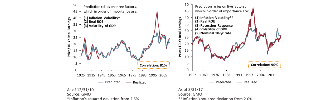
The behavioral model’s explanatory power for S&P 500 P/E improved from an 81% correlation in the early version (1925–2006) to 90% in the revised version (1962–2017), precisely capturing extreme market valuation points.

2. Quantitative Validation and Counterexamples of “Unchanging Human Nature”

Mr. Murray argues that “unchanging human nature” is the primary driver of market volatility. This view finds partial support in behavioral finance but requires more nuanced definition.

• Supporting Evidence: Behavioral finance concepts such as the “disposition effect” (selling winners too early and holding losers too long) and “herding” have been repeatedly validated across a century of market data. For instance, Shiller (1981) showed that stock price volatility far exceeds what can be explained by the present value of future dividends, with the excess volatility attributable to the contagion of investor sentiment.
• Counterexamples and Refinements: However, the specific manifestations of “human nature” change with institutional evolution. For example, the 1987 “Black Monday” crash was partly driven by mechanical selling from “portfolio insurance” strategies, rather than pure emotional panic. This represents a new form of “technical weakness”—a variant of the “old-fashioned excesses” Mr. Murray describes in the computer age. Thus, human nature has not changed, but it amplifies its impact through new tools (algorithms, leveraged ETFs).

3. Revisiting the “Always Hold Stocks” Strategy

Mr. Murray advises investors to “always maintain some interest in common stocks” to avoid the “psychological bankruptcy” of missing subsequent gains after fully exiting. This advice is valid over the long term but requires dynamic adjustment based on valuation levels.

• Data Comparison: The table below shows differences in real annualized returns over 10 years for investments initiated at different valuation intervals (using Shiller CAPE as a reference).

Starting Valuation Range (Shiller CAPE)	Example Starting Year	Subsequent 10-Year Real Annualized Return (S&P 500)	Strategy Implication
Very Low (< 10)	1920, 1932, 1949	Approximately 10% – 15%	Should be heavily invested
Moderate (15 – 20)	1950, 1984, 2003	Approximately 5% – 8%	Maintain neutral allocation
Very High (> 25)	1929, 1999, 2021	Approximately -2% to 2%	Significantly reduce, but not fully exit

• New Perspective: Mr. Murray’s advice is most applicable in the “moderate valuation” range. At extreme high valuations (e.g., the 1999 internet bubble), fully exiting, while missing the final leg of the rally, avoids a subsequent decade of negative or low returns. The core value lies in preventing investors from making worse decisions (chasing highs) due to “fear of missing out,” rather than mechanically requiring full investment at all times.

4. Supplement on GMO and Jeremy Grantham

The GMO statement and Grantham’s background at the end of the cited passage provide a modern footnote to the above discussion.

• Strategy Consistency: Grantham is known for long-term value investing and “mean reversion” predictions. GMO’s assumed 5.75% real return is based on statistical analysis of long-term historical returns (such as the 1871–1954 data cited by Murray), with the view that current (2017) high valuations will cause future returns to revert to that mean. This subtly contrasts with Mr. Murray’s warning that “historical patterns may fail.”
• New Evidence: Grantham himself has successfully predicted market bubbles multiple times (e.g., 2000 tech stocks, 2008 real estate). His success partly stems from identifying what Mr. Murray called “new conditions”—the “new economy” narrative in 2000 and the “subprime securitization” structure in 2008—which were new “excesses” emerging after old patterns failed. This proves that understanding the underlying logic of “unchanging human nature” (greed and fear) and identifying its specific manifestations under “new conditions” is the core of investment analysis.

Summary: This cited passage reveals an eternal dilemma in investment analysis: we rely on historical data to build models, yet the evolution of market conditions inevitably renders those models obsolete. Mr. Murray’s wisdom lies in acknowledging the limitations of models while holding firm to insights into human weaknesses. The task for modern investors is not to find a permanent formula, but, like Grantham, to continuously identify the new disguises of human weakness under “new conditions,” building on an understanding of historical patterns.