New Options for Equity Investors

Theme and Background

This chapter explores the volatility characteristics of long-term returns in the U.S. stock market and the challenges they pose to investors. The report notes that since the late 19th century, the annual real return of the U.S. stock market has been approximately 6.5%. However, due to high volatility, returns tend to occur in sharp and irregular fluctuations rather than steadily meeting expectations. Current market valuations are elevated, and the outlook for real returns over the next seven years is poor, leaving investors with the challenge of capturing the equity risk premium in an expensive market.

Core Thesis

The author's core investment argument is: The equity risk premium can be captured through stock index options (particularly by selling put options), and this approach is less dependent on market valuations. The counterintuitive finding is that, since 1983, nearly all of the excess return of the S&P 500 has come from exposure to downside risk (i.e., selling put options), rather than upside risk (buying call options). Traditional risk metrics (such as volatility and beta) cannot explain this phenomenon. Investors are actually compensated for correlated downside risk, not statistical volatility.

Key Arguments and Data

1. Volatility of Long-Term Returns: Exhibit 2 shows that rolling 7-year real returns have experienced periods of deviation from the equilibrium level lasting over a decade, including both bear markets far below 6.5% and bull markets far above the mean. Predictive models based on Shiller's Cyclically Adjusted Price-to-Earnings ratio (CAPE) indicate that when the market is overpriced, future 7-year returns tend to be poor; current valuations suggest a bleak near-term outlook.

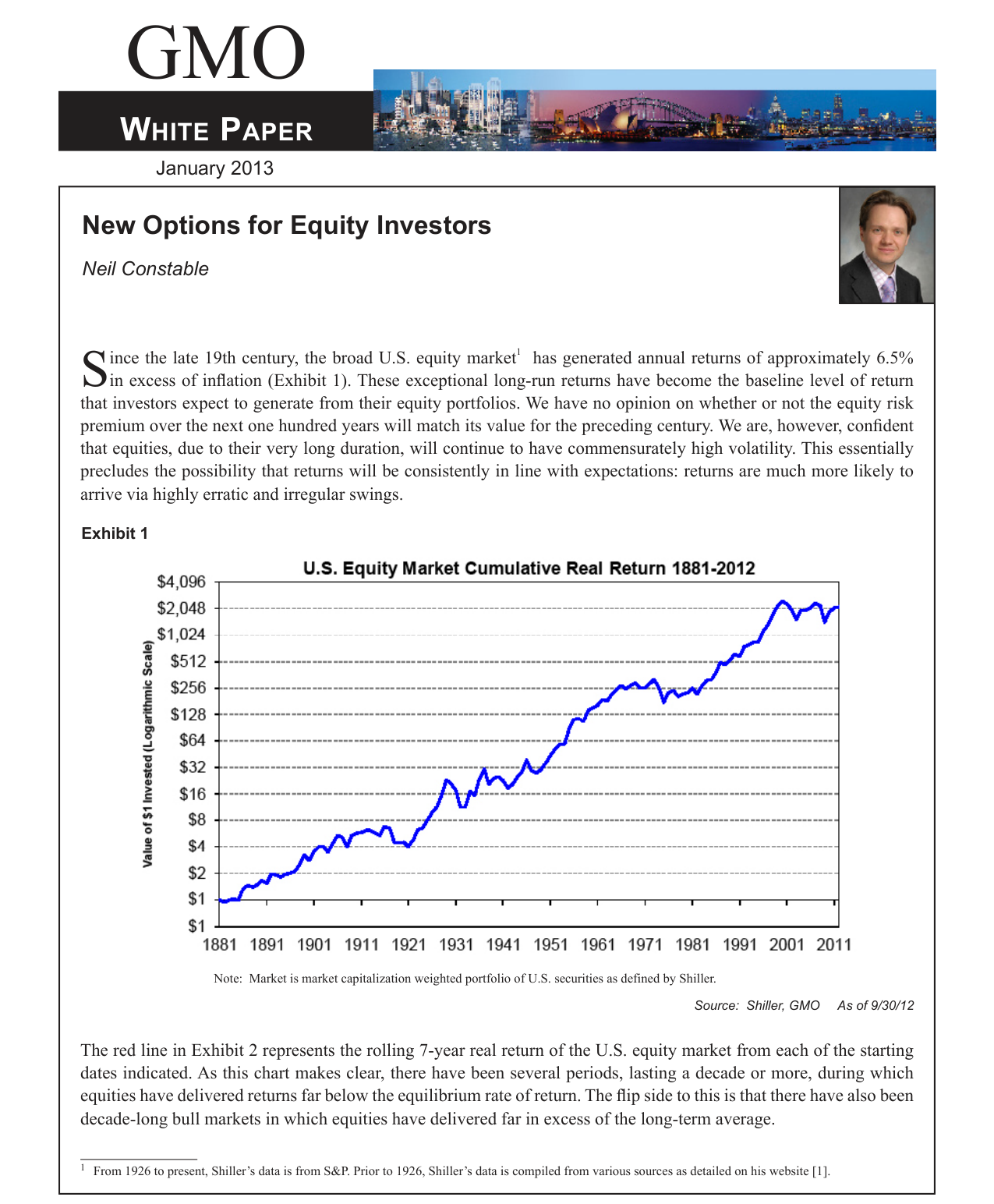
The cumulative real return of the U.S. stock market grew from $1 in 1881 to approximately $2,048 in 2012 (log scale), with a long-term annualized excess return of about 6.5%

2. Option Decomposition Analysis: Using put-call parity, the report decomposes market returns into three components: cash, selling put options, and buying call options. The analysis covers the period from March 1983 to October 2012, using 1-month at-the-money (ATM) S&P 500 option data.

3. Key Findings: Exhibit 4 shows that, after transaction costs, nearly all of the excess return of the S&P 500 comes from selling put options (downside exposure), while buying call options (upside exposure) contributes negatively to returns. The specific data is as follows:

Metric	Selling Put Options	Buying Call Options
Annualized Return (after costs)	Close to overall market return	Net drag
Monthly Return Standard Deviation	Similar	Similar
Maximum Single-Month Loss	Limited	-4.5% (September 2008)
Beta	Similar	Similar

Note: Buying call options incurred a single-month loss of 4.5% in September 2008 (after the Lehman Brothers bankruptcy) due to paying a high premium.

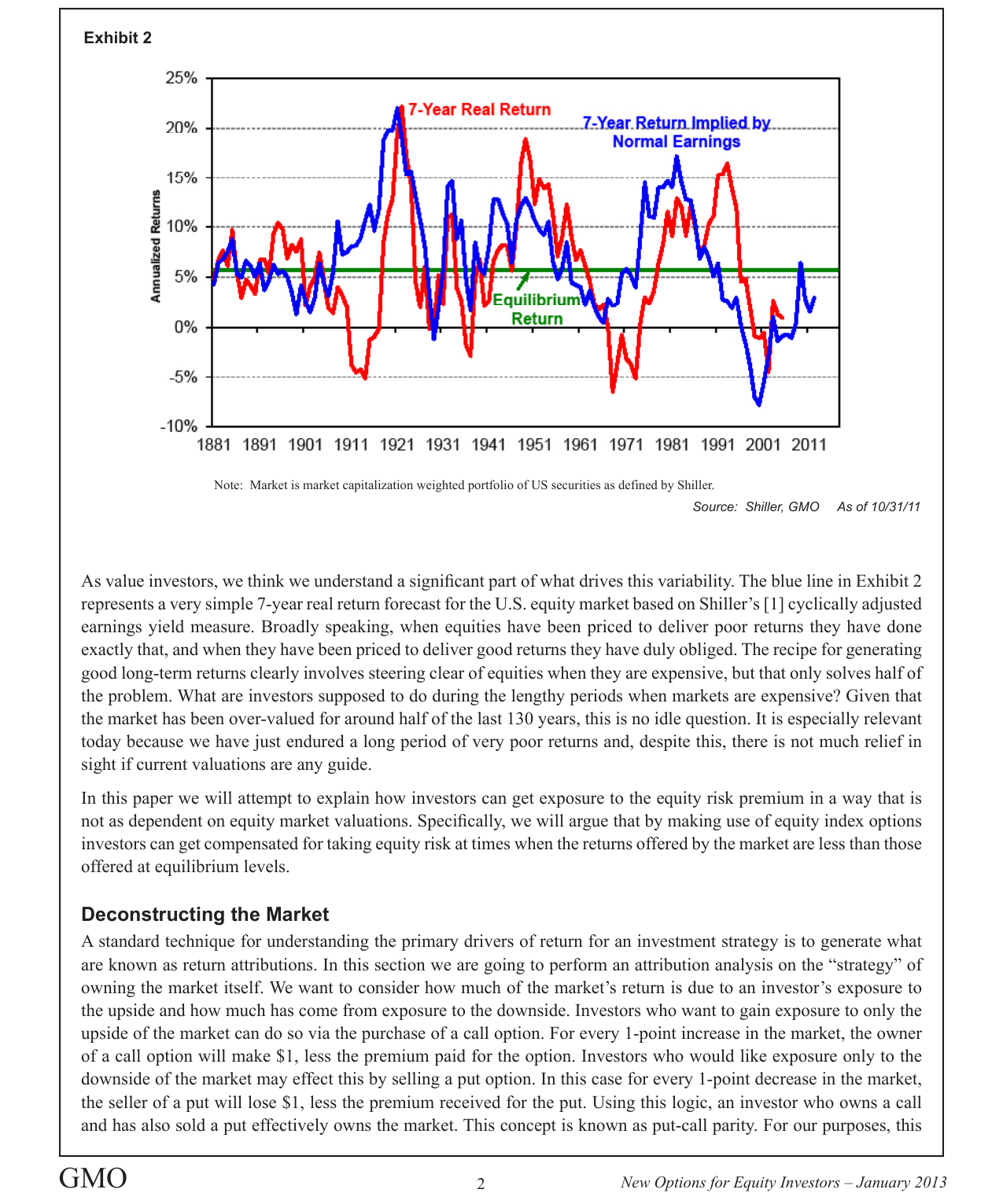
Between 1881 and 2011, the 7-year real return of U.S. stocks (red line) and the return implied by normal earnings (blue line) fluctuated significantly, with a long-term equilibrium return of approximately 5% (green line)

4. Mismatch of Risk and Return: Traditional risk metrics (volatility, beta) suggest that selling puts and buying calls should have similar returns, but the actual results are starkly different. The author argues that investors are actually compensated for drawdown risk—the risk exposure during the market's largest single-day or single-month losses—rather than statistical volatility.

Companies/Assets Involved

• S&P 500 Index: The core underlying asset of the analysis, representing the U.S. large-cap stock market.
• Option Instruments: 1-month at-the-money S&P 500 put and call options. Data sources include the CME (futures options from 1983-1996) and the Option Metrics Ivy database (index options from 1996 onwards).
• Cash Asset: 3-month U.S. Treasury bills (T-bills), used to collateralize the put options.

Investment Implications

• Selling Put Options Strategy: When valuations are high and the outlook for traditional buy-and-hold returns is poor, investors can capture the equity risk premium by selling put options, as historical data shows that downside risk exposure is the primary source of market returns.
• Avoid Traditional Risk Metrics: Investors should not rely on volatility or beta to measure risk compensation but should instead focus on drawdown risk and correlated downside risk.
• Current Market Application: Given that current valuations remain high, traditional stock investment returns may be limited. Option strategies, particularly selling puts, offer an alternative that is less dependent on valuations.

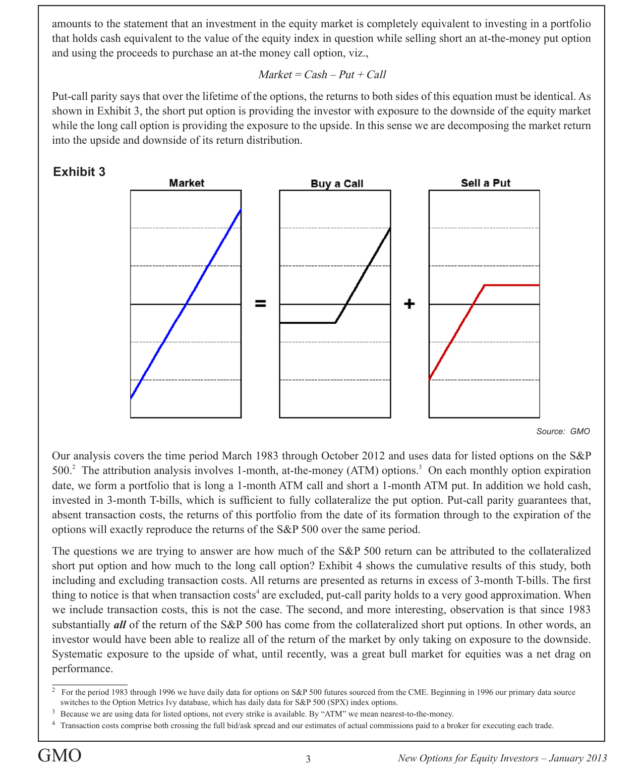
Illustration of the put-call parity relationship: Market returns (left) can be decomposed into a combination of buying call options (center) and selling put options (right)

Additional Arguments and Perspectives

1. The "Implied-Realized Volatility Gap" in Option Pricing as a Risk Compensation Mechanism

The follow-up analysis further reveals the source of long-term returns for option sellers: the gap between implied volatility and realized volatility. Data shows that the implied volatility of 1-month ATM put options is, on average, 2.7% higher than the subsequent 30-day realized volatility (Exhibit 7). This gap is not evidence of market inefficiency but rather a fair price for unhedgeable tail risk (such as the 1987 Black Monday crash).

Key Comparison:

Risk Type	Option Seller Bears	Traditional Stock Holder Bears
Market Crash Risk	Yes (compensated via the gap)	Yes (compensated via the equity risk premium)
Volatility Risk	Yes (but not the primary compensation source)	Yes (but no specific compensation)
Valuation Risk	Low (returns are insensitive to valuations)	High (returns are negatively correlated with valuations)

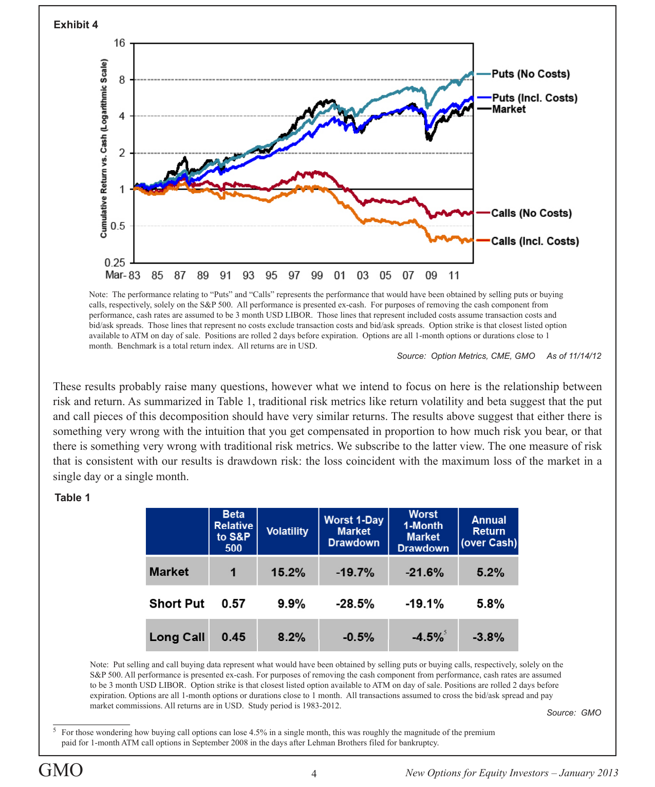
Between 1983 and 2012, the cumulative return of selling put options (costless) reached approximately 8x, significantly outperforming the market (about 5x), while the cumulative return of buying call options (including cost) was only about 0.3x

2. Quantitative Evidence of the Insensitivity of Option Seller Returns to Market Valuations

Exhibit 6 shows the decomposition of 7-year returns, sorted by starting valuation based on the Shiller CAPE yield, for the period 1983-2012. The core findings are:

• Put option sellers had 7-year returns that were below cash in only a very few rolling periods (red dots in Exhibit 6).
• Call option buyers had returns that were highly negatively correlated with starting valuations, making them the primary source of losses when the market was overvalued.
• TMT Bubble Case: During the extreme valuation period (low CAPE yield), put sellers significantly outperformed both call buyers and market holders.

3. Decomposition Formula for Expected Returns and Market Equilibrium Mechanism

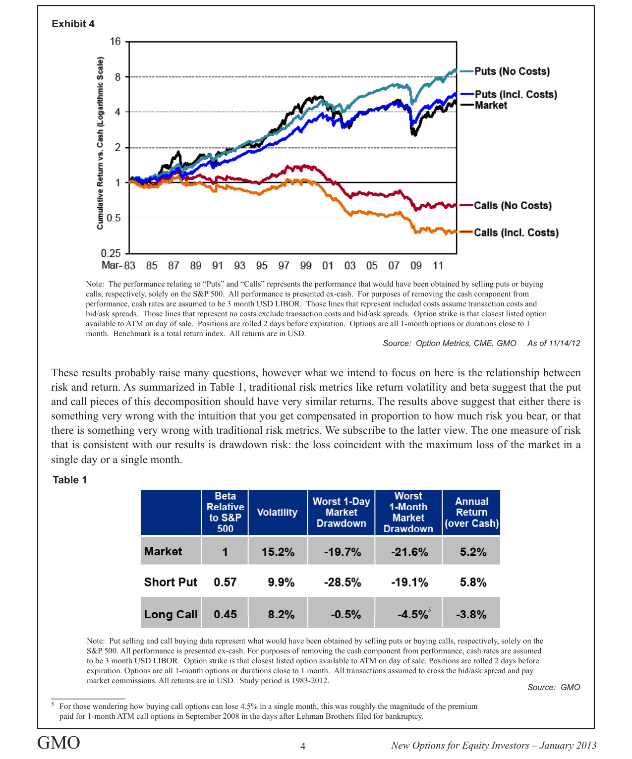
Selling put options (Short Put) had an annualized return of 5.8%, higher than the market's 5.2%, with a volatility of 9.9%, significantly lower than the market's 15.2%, and a maximum monthly drawdown of -19.1%, better than the market's -21.6%

The follow-up analysis introduces Figelman's decomposition formula:

```

Expected Return = ½(Expected Market Return) + (Expected Implied-Realized Volatility Gap)

```

Where:

• The ½ factor stems from the delta of a short-term ATM put option being approximately 0.5.
• The gap is the compensation to the option seller for unhedgeable crash risk.
• This gap adjusts automatically in long-term equilibrium, causing the expected returns of put sellers and market holders to converge.

4. Practical Implications for Portfolio Construction

The follow-up analysis introduces the concept of opportunity set expansion:

Strategy	Condition for Attractiveness	Nature of Risk
Selling Put Options	High insurance premium (high implied volatility)	Crash risk
Holding Stocks	High earnings yield (low CAPE)	Valuation risk

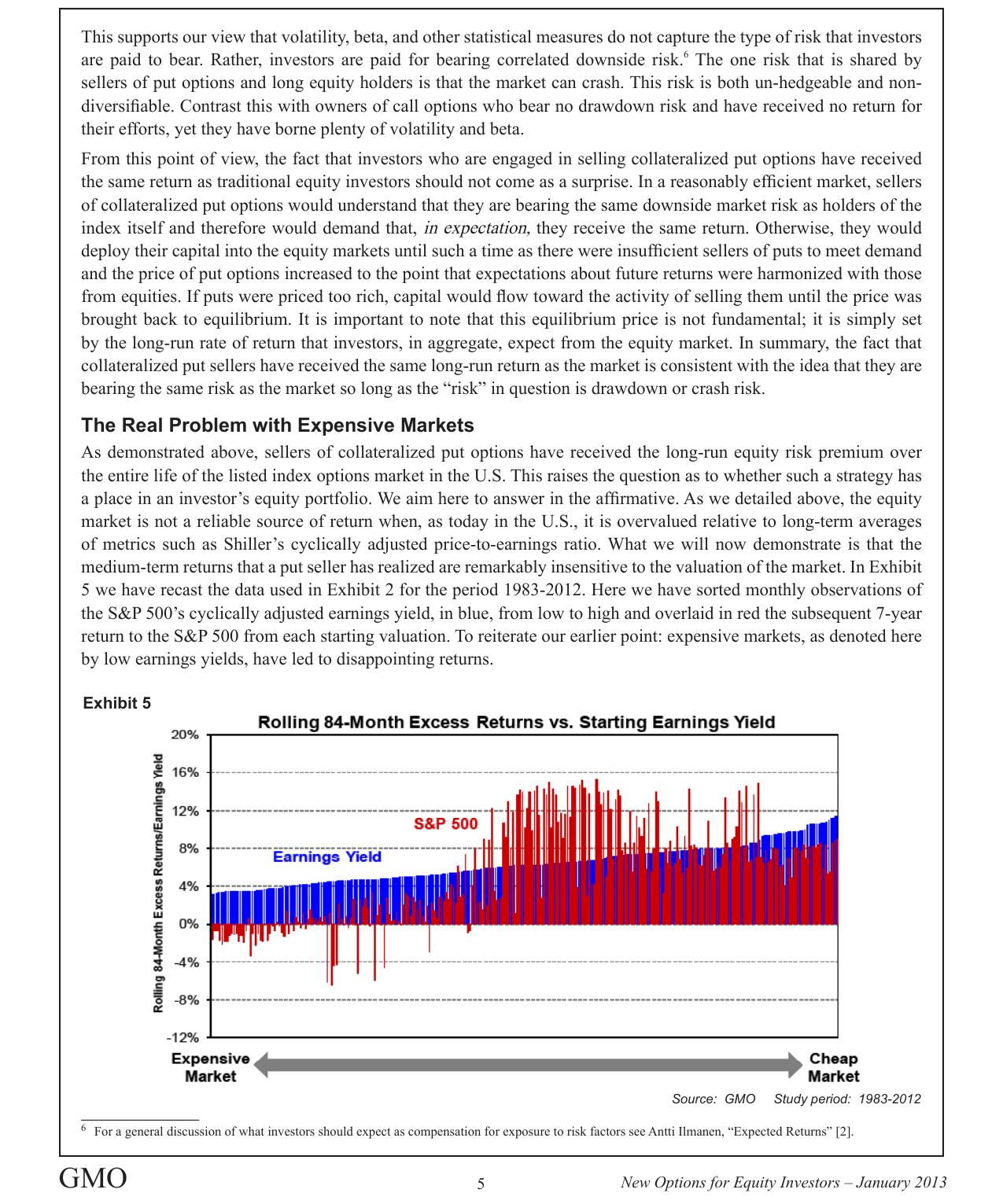
Data from 1983-2012 shows that the lower the starting earnings yield (expensive market, left), the worse the subsequent 7-year excess return (red bars); a high earnings yield (cheap market, right) is accompanied by high returns

These two conditions do not necessarily occur simultaneously, so investors can achieve risk diversification through dynamic allocation. For example, during the TMT bubble in 2000, the CAPE was over 40, but implied volatility was also high, making selling put options a superior strategy to holding the index.

5. Redefining "Market Efficiency"

The follow-up analysis refutes the view that "the gap is market inefficiency," proposing that:

• If the gap is too large, capital flows into put selling, pushing the price down to equilibrium.
• If the gap is too small, put sellers exit, pushing the price up to equilibrium.
• The equilibrium price is not determined by "fundamentals" but is set by the collective expectations of investors regarding long-term equity returns.

This mechanism explains why, between 1983 and 2012, put sellers and market holders achieved the same long-term returns—both bear the same downside market risk.

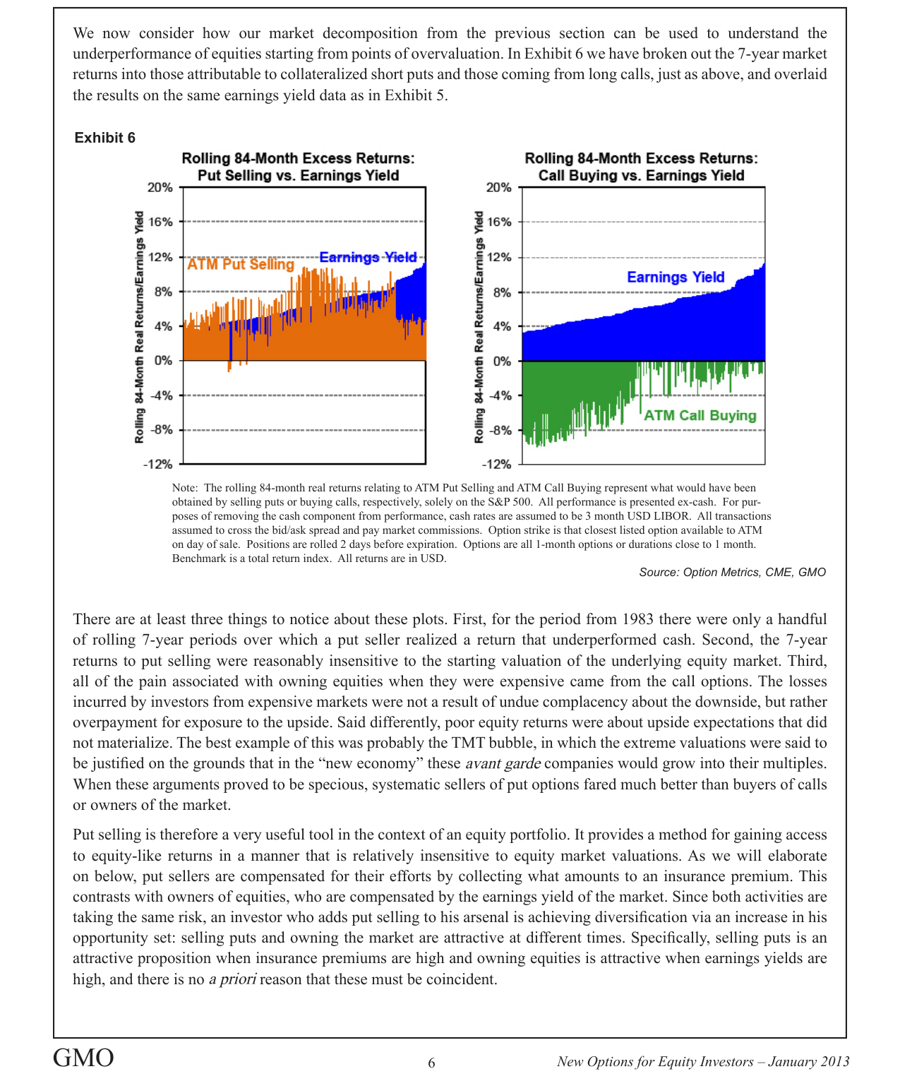
The left chart shows that selling put options maintains positive returns across all valuation levels (orange), while the right chart shows that buying call options generates significant negative returns in expensive markets (left, green)

This is an analysis of the follow-up content to the "Introduction," continuing the previous style and supplementing new arguments, data, and perspectives.

Additional Analysis: Implied Volatility as a Timing Indicator and the Quantitative Anchoring of the Variance Risk Premium (VRP)

The core contribution of this paper is that it not only proposes the put selling strategy but also provides a quantifiable timing framework for it, ultimately unifying the expected return of this strategy with the traditional equity risk premium (ERP) in theory.

1. Empirical Evidence for Implied Volatility as a Timing Indicator

The author uses empirical data (Exhibit 8, 1996-2012) to verify the predictive power of implied volatility (IV) for the future "implied-realized volatility difference" (i.e., the put premium). They divide the implied volatility of 1-month ATM put options into five quintiles and observe the subsequent 30-day actual difference.

• Core Finding: When implied volatility is high (e.g., after a market panic), the subsequent "implied-realized volatility difference" also tends to be larger. This provides a clear action guide for value investors: sell options when implied volatility is high (i.e., when "fear" is at its peak), similar to an insurance company raising premiums before a hurricane season.
• Analogy to Stock Valuation: The author cleverly draws an analogy to Shiller's CAPE. Just as CAPE is a starting point for judging the attractiveness of the stock market, implied volatility is a starting point for judging the attractiveness of selling options. Their low correlation forms the basis for strategy diversification.

2. Quantification and Theoretical Unification of the Variance Risk Premium (VRP)

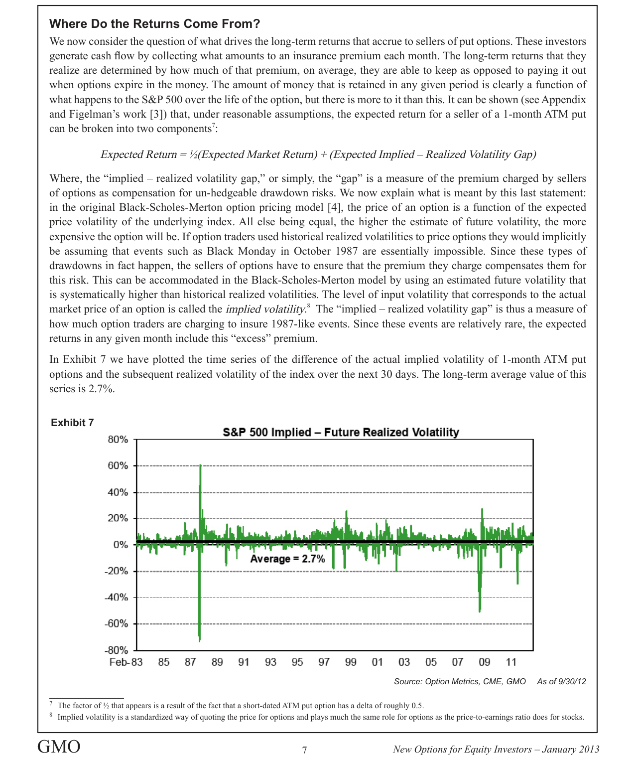
From 1983 to 2012, the long-term average difference between S&P 500 implied volatility and future realized volatility was 2.7%, with the gap exceeding 60% during the October 1987 crash

The appendix provides the most profound theoretical insight of the paper, mathematically linking the expected return of the put selling strategy to the ERP.

• Equivalence Principle: The author proposes that a fully collateralized short put position bears the same downside risk (drawdown risk) as a direct long index position. Therefore, over the long term, the expected returns of both should be equal. This principle is expressed by the formula: `E(-P) = μtS`, where `E(-P)` is the expected return from selling the option, `μ` is the market's expected drift rate (i.e., the ERP), `t` is time, and `S` is the spot price.
• Determination of VRP: Based on this principle, the author deduces that the expected "implied-realized volatility difference" (i.e., the variance risk premium, VRP) is determined by the ERP. In other words, the VRP is not an independent risk premium but another manifestation of the ERP in the options market.
• Data Validation: The author substitutes a 6.5% annualized ERP into the formula and calculates a 1-month expected VRP of 2.4%. This theoretical value is highly consistent with the historical actual average shown in Exhibit 7. This provides strong empirical support for the assertion that "the long-term return of the put selling strategy equals the ERP."

3. Comparative Data: Theoretical VRP vs. Historical VRP

Metric	Value	Source/Explanation
Annualized Equity Risk Premium (ERP)	6.5%	The author's assumed long-term expected market return
Theoretical 1-Month VRP	2.4%	Calculated from the formula `μt` (6.5% / 12)
Historical Average 1-Month VRP	~2.4%	Empirical result based on 1996-2012 data (Exhibit 7)

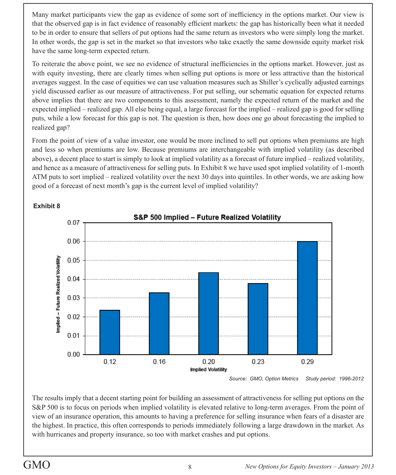
Grouped by implied volatility quintiles, the volatility premium in the highest group (0.29) reached approximately 6%, while in the lowest group (0.12) it was about 2.4%, indicating that option sellers receive a higher insurance premium during periods of high panic

Conclusion: The high consistency between the theoretical and historical values proves that the VRP is not a product of market irrationality but a result of rational pricing, with its magnitude precisely compensating the option seller for bearing the same systematic risk as a stock holder.

4. Final Positioning of the Strategy: Diversification of the Opportunity Set, Not Diversification of Risk

In the conclusion, the author clearly distinguishes between two types of "diversification":

• Diversification of Risk (via risk reduction): This is the goal of traditional portfolio construction. The author emphasizes that selling put options cannot achieve this, as it shares the same drawdown risk as a long stock position.
• Diversification of the Opportunity Set: This is the core value of the strategy in this paper. It provides another independent dimension (implied volatility) for assessing whether bearing stock downside risk is worthwhile. When stocks are expensive (high CAPE), expected market returns are low; however, implied volatility may be high due to market panic, making selling options very attractive. The opposite is also true.

Final Conclusion: The put selling strategy is not a risk hedging tool but an income enhancement tool. It offers investors an alternative way to capture returns commensurate with stock risk (i.e., the ERP) when traditional stock valuations are uninformative.